6. Multispectral Imagery#
This lab introduces how to visualize and process multispectral and multiband imagery using Landsat satellite data.
Introduction to Landsat Imagery#
The Landsat program is a joint NASA and USGS program and the longest running satellite imagery enterprise in the U.S. and the world. The program has so far launched 9 satellites since 1972 with Landsat 1 through 2021 with Landsat 9. The spatial resolution varies from 15 to 100 m, and the temporal resolution (meaning the time it takes for the same location to be photographed) is approximately 16 days. Landsat imagery is divided into scenes each measuring approximately 185 x 185 km.
The main instrument consists of a multispectral scanner that records data in separate bands. The specific wavelength ranges differ across missions, but the multispectral scanners typically record information across the visible (blue, green, red), near infrared (NIR), short wave infrared (SWIR), and thermal infrared (TIR) spectrum.
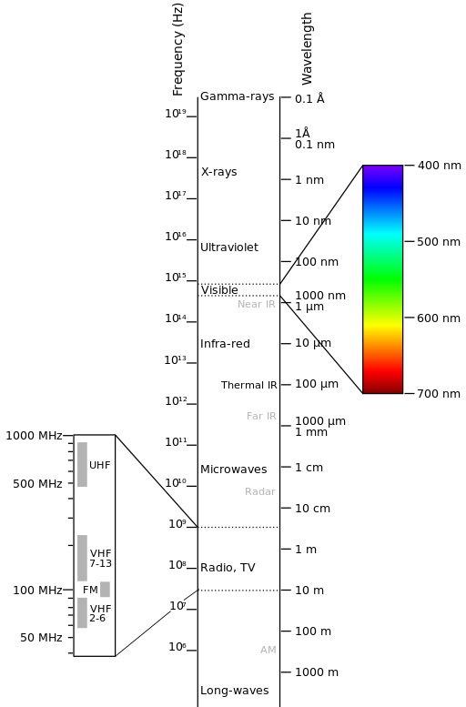
Photo credit: Victor Blacus
The most recent Landsat missions (7, 8, and 9) have the highest quality data. The bands and their corresponding wavelengths are shown below.
Landsat-7 ETM+ Bands (µm) |
Landsat-8 OLI and TIRS Bands (µm) |
Landsat 9 OLI and TIRS-2 Bands (µm) |
||||
|---|---|---|---|---|---|---|
30 m Coastal/Aerosol |
0.435-0.451 |
Band 1 |
0.433-0.453 |
|||
Band 1 |
30 m Blue |
0.441-0.514 |
30 m Blue |
0.452-0.512 |
Band 2 |
0.450-0.515 |
Band 2 |
30 m Green |
0.519-0.601 |
30 m Green |
0.533-0.590 |
Band 3 |
0.525-0.600 |
Band 3 |
30 m Red |
0.631-0.692 |
30 m Red |
0.636-0.673 |
Band 4 |
0.630-0.680 |
Band 4 |
30 m NIR |
0.772-0.898 |
30 m NIR |
0.851-0.879 |
Band 5 |
0.845-0.885 |
Band 5 |
30 m SWIR-1 |
1.547-1.749 |
30 m SWIR-1 |
1.566-1.651 |
Band 6 |
1.560-1.660 |
Band 6 |
60 m TIR |
10.31-12.36 |
100 m TIR-1 |
10.60-11.19 |
Band 10 |
10.30-11.30 |
100 m TIR-2 |
11.50-12.51 |
Band 11 |
11.50-12.50 |
|||
Band 7 |
30 m SWIR-2 |
2.064-2.345 |
30 m SWIR-2 |
2.107-2.294 |
Band 7 |
2.100-2.300 |
Band 8 |
15 m Pan |
0.515-0.896 |
15 m Pan |
0.503-0.676 |
Band 8 |
0.500-0.680 |
30 m Cirrus |
1.363-1.384 |
Band 9 |
1.360-1.390 |
Earlier missions (Landsat 1-5) might be useful for historic purposes, and their bands and corresponding wavelengths are available here. The Landsat 6 mission failed to reach orbit.
Download Imagery#
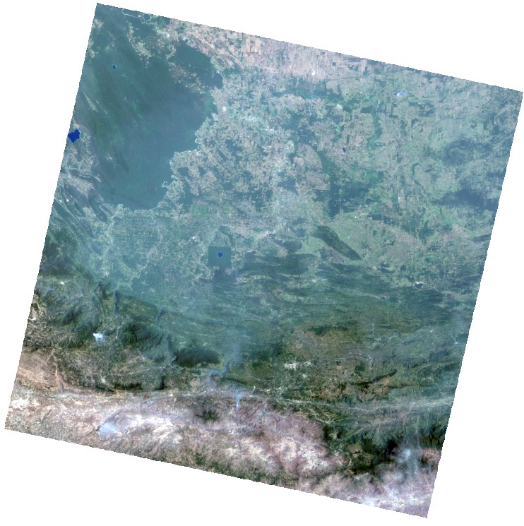
Imagery can be downloaded from USGS Earth Explorer. Under Search Criteria, identify an area of interest and filter by Cloud Cover (under 10%). Under Data Sets, select Landsat Collection 2 Level-2 and Landsat 8-9 OLI/TIRS C2 L2, then click on Results. For this exercise, we will work with Landsat imagery around 16° 20’ 23’’ N and 90° 38’ 27’’ W. The Landsat 8 imagery acquired on 2017/4/3 is of a high quality with low cloud cover. Click on Product Options and download the Product Bundle. Extract all of the files to your desired folder.
This folder should contain several Geotiff files and metadata. Each band is stored as a separate Geotiff file. To view band combinations, we will have to load these bands together as a single composite, multiband image.
In ArcGIS Pro, we just have to add the combined .txt file or Raster Product (usually ______MTL.txt). We can then alter the visualization and band combination under Symbology.
In QGIS, we have to build a virtual raster. Go to Raster -> Miscellaneous -> Build Virtual Raster. Under Input layers, we will add only the 30 meter bands listed in the chart above: Bands 1, 2, 3, 4, 5, 6, 7, and 9, in order. Set Resolution to Highest and Place each input file into a separate band. The visualization and band combination can be edited under the Properties of the Virtual raster. Bilinear Resampling and an updated canvas (DRA in ArcGIS Pro) can improve visualization.
Landsat 8 and 9 data are delivered in a 16-bit unsigned format, while earlier Landsat imagery is delivered in an 8-bit unsigned format. To convert these digital numbers to reflectance values, refer to scale factors provided by the USGS. For Landsat 8 and 9, the scale factor is 0.0000275 with an offset of -0.2. In Raster Calculator, we can use the following expression:
"16-bit raster" * 0.0000275 - 0.2
The values should be between 0 and 1, which multiplied by 100 gives the percent reflectance (0% to 100%). Some values may fall below 0 and above 1, representing an overcorrection for atmospheric effects. If necessary, these values can be removed using a conditional expression using Raster Calculator in ArcGIS Pro (Con) or QGIS (if):
Changing negative values to zero:
Con("Reflectance raster" < 0, 0, Con("Reflectance raster" > 1, 1, "Reflectance raster"))
if("Reflectance raster" < 0, 0, if("Reflectance raster" > 1, 1, "Reflectance raster"))
Changing negative values to NoData:
Con("Reflectance raster" < 0, 0/0, Con("Reflectance raster" > 1, 1, "Reflectance raster"))
if("Reflectance raster" < 0, 0/0, if("Reflectance raster" > 1, 1, "Reflectance raster"))
Adding the absolute value of the minimum value to the raster (my preferred method):
"Reflectance raster" + "Minimum Value"
Band Compositing#
Multiband imagery can be visualized with different band combinations using the red, green, and blue additive color model. In this system, 3 bands can be viewed at one time, each displayed as red, green, or blue. A fourth channel, alpha, can be optionally blended on top of the 3 traditional bands.
Band composites can be referenced with the 3 numbers each representing the relevant band, in order of red, green, or blue. The band combination 4-3-2, therefore, indicates that Band 4, Band 3, and Band 2 will be displayed as red, green, and blue, respectively. In Landsat 8 and 9, Band 4 is red, Band 3 is green, and Band 2 is blue, meaning that when displayed as 4-3-2, we are viewing the visible spectrum or true color of the image.
Different materials, for example, vegetation, water, soil, rock, etc., reflect the electromagnetic spectrum differently. Spectral reflectance is the ratio of the amount of light reflected by a surface to the amount of light that hits it at different wavelengths. A spectral reflectance curve shows the variations in spectral reflectance across different wavelengths and materials.
The following spectral reflectance curves show reflectance values for different materials at different wavelengths and Landsat bands (Landsat 7 above and Landsat 8 and 9 below):
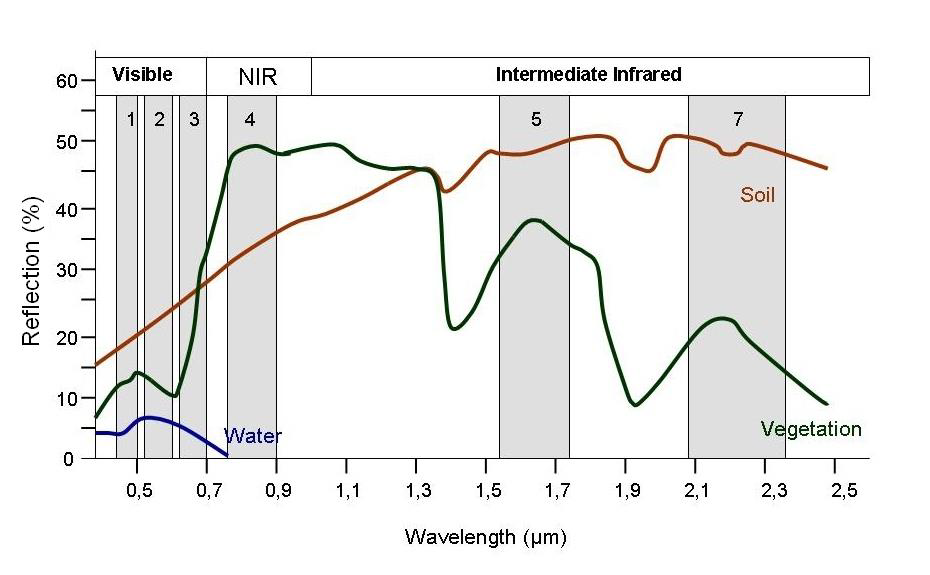
Photo credit: SEOS eLearning
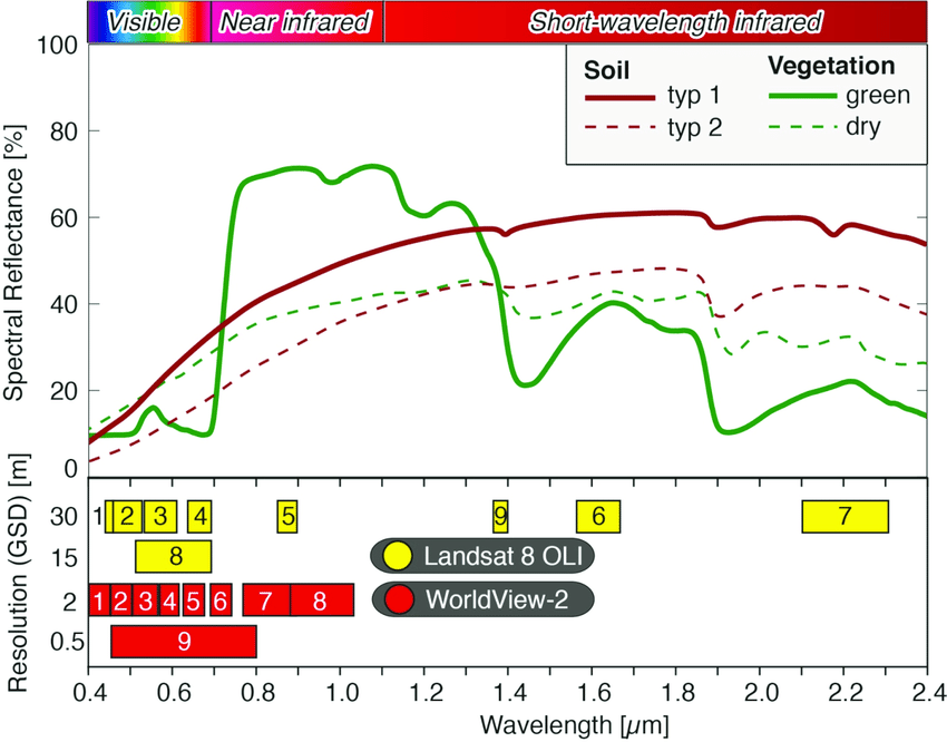
Photo credit: Wulf et al. 2015
Here are some useful band combinations in Landsat 8 and 9:
Natural Color |
4-3-2 |
Shortwave Infrared (Urban) |
7-6-4 |
Color Infrared (Vegetation) |
5-4-3 |
Agriculture |
6-5-2 |
Atmospheric Penetration |
7-6-5 |
Healthy Vegetation |
5-6-2 |
Land/Water |
5-6-4 |
Natural with Atmospheric Removal |
7-5-3 |
Shortwave Infrared |
7-5-4 |
Vegetation Analysis |
6-5-4 |
Geology |
7-6-2 |
Bathymetric |
4-3-1 |
Forest Fires |
7-5-2 |
Bare Earth |
6-3-2 |
Vegetation/Water |
5-7-1 |
Archaeology (Parcak/Egypt) |
5-4-3 |
Archaeology (Saturno/Guatemala) |
5-3-2 |
See also: ESRI, NV5, GIS Geography, Open Weather
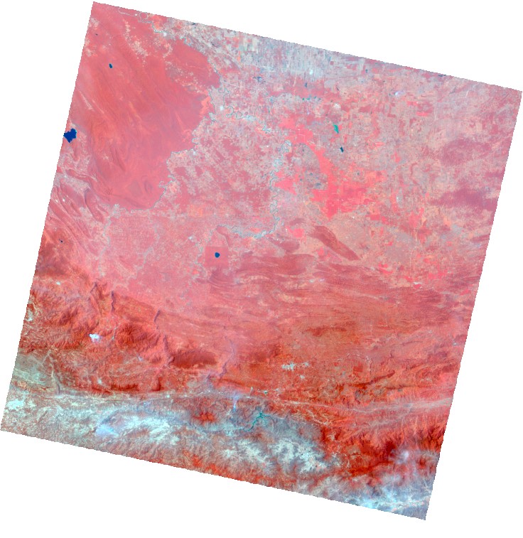
Here is a false color composite using Bands 5-3-2:
Band Ratios#
Computing band ratios can also highlight features. Band ratios are calculated by dividing a band with a high reflectance value for a specific material by the band with a low reflectance value for that same material using Raster Calculator (especially when the ratios for other materials will be neutral). In Landsat 8, the Band 5 / Band 4 ratio will highlight vegetation, Band 7 / Band 1 will highlight soil, and Band 1 / Band 5 or Band 2 / Band 6 will highlight water.
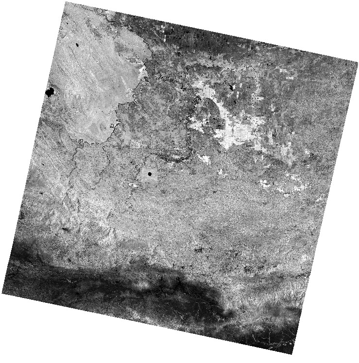
Here is a ratio of Band 5 / Band 4, with vegetation on the white end of the color scheme:
Band ratios can also eliminate issues discerning features in high shadow areas. In the following image deciduous and coniferous forest have different spectral reflectance in sunlit vs. shaded areas, but when the ratio is calculated, this discrepancy is fixed.
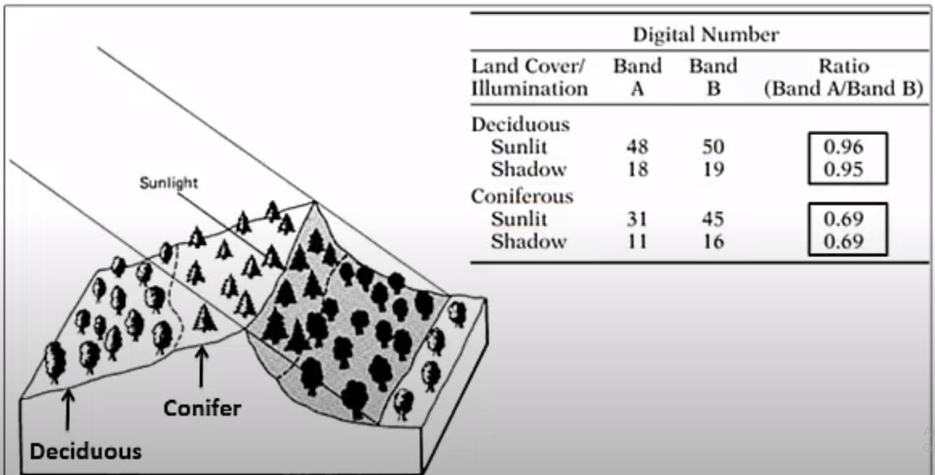
Photo credit: Middlebury Remote Sensing
Raster Calculator in QGIS or ArcGIS Pro can be used to calculate these ratios.
Vegetation indices (NDVI)#
Building off the idea of band ratios, several indices can be calculated by performing map algebra to combine different bands. The Normalized Difference Vegetation Index (NDVI) is an example that transforms multiband data into a single raster that represents no vegetation (-1) to high vegetation (1).
In ArcGIS Pro, the NDVI can be calculated by selecting the .txt file of combined bands in the Contents, going to Imagery, clicking the Indices dropdown, and selecting NDVI.
Alternatively, we can calculate the NDVI in Raster Calculator using the following formula:
We can visualize the NDVI with a green color scheme.
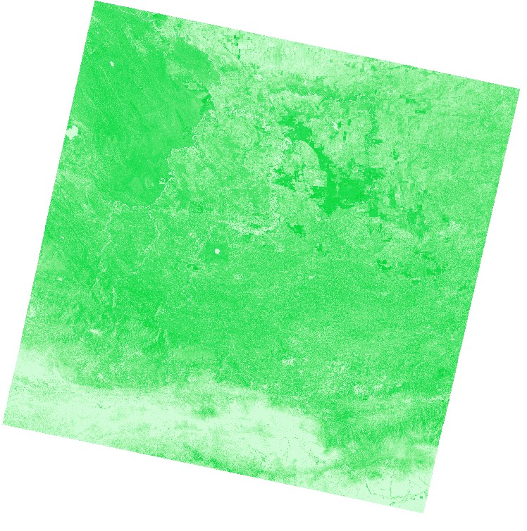
Or we can use a green color scheme with values under 0 (water) set to blue. Here is an example color scheme for QGIS: (ndvi.txt)
Principal Component Analysis#
Principal components analysis calculates variability through several iterations, with each iteration showing less variability.
In ArcGIS Pro run the Principal Components Analysis tool by loading the individual raster bands and selecting the number of principal component iteration (this value should match the number of inputs). Change the output to a folder rather than a geodatabase, and do not enter a filetype extension after the filename if you want to produce a raster for each iteration. The tool will load a new multiband raster containing all the principal components. You can manually load each individual component from the same folder.
In QGIS, go to Plugins, Manage and Install Plugins, search for Semi-Automatic Classification Plugin, and install. There should now be an SCP menu in QGIS (try restarting QGIS if you don’t see it). If you receive an error message, you may need to upgrade some dependencies. If so, exit out of QGIS, and in Windows, open the OSGEO4W Shell and run the following command:
pip3 install --upgrade remotior-sensus scikit-learn torch
On a Mac, the SCP plugin does not work on the latest version of QGIS. You will have to install an older version of QGIS, for example, QGIS 3.34. Other long-term release versions are available here. Once installed, locate the folder path where you have QGIS 3.34 installed. You will have to right-click QGIS 3.34 in Applications, and select Show Package Contents. Navigate through the folders to locate the Python and pip3 installations. The folder should be something like /Applications/QGIS-LTR.app/Contents/MacOS/bin. Verify that this is the correct folder, if not modify the below code to match the correct folder structure.
Open the Mac Terminal and copy the following, then press Enter:
/Applications/QGIS-LTR.app/Contents/MacOS/bin/pip3 install --upgrade remotior-sensus scikit-learn torch
If prompted, install command line developer tools, agree to the license statement, and run the above code again.
Then run the following:
/Applications/QGIS-LTR.app/Contents/MacOS/bin/pip3 install numpy==1.26.4
And finally run the following:
/Applications/QGIS-LTR.app/Contents/MacOS/bin/pip3 install --upgrade remotior-sensus
Under SCP, click Band Set. From the Single band list, load the individual bands (you may need to click refresh and make sure the bands are in your Layers contents). Each band is weighted equally (1) by default. In this case, our rasters all have the same range, so we do not need to weigh them.
Click Band Processing, then PCA, select Number of Components and choose a number of iterations. Click Run.
Note that ArcGIS Pro and QGIS may produce different results, but variability will decrease with each iteration.
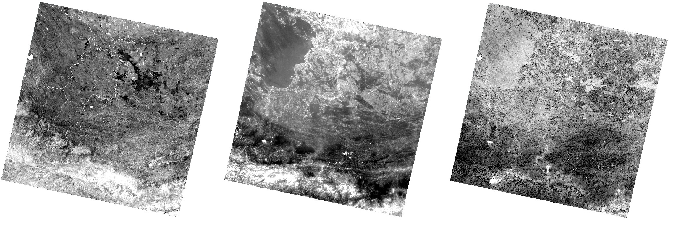
The following image shows the first order PCA, second order PCA, and third order PCA from left to right.
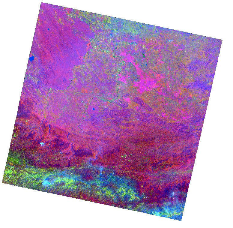
The following image shows the PCA composite, with PCA1, PCA2, and PCA3 shown as RGB.
Texture Analysis#
Texture analysis is used in remote sensing to highlight differences between materials. In QGIS, the GRASS tool r.texture calculates several metrics, variance being the most common method used.
Run r.texture, select the input raster, select Textural Measurement Method(s) (var = variance), select size of moving window (must be an odd integer, 3 is the default), and choose an output folder. Note that this tool inputs the folder as a string, so do not use any spaces in your folder path, or put the folder path in quotes.
The following image is a texture (variance) analysis of the first order Principal Component Analysis, highlighting the differences between different types of land cover:
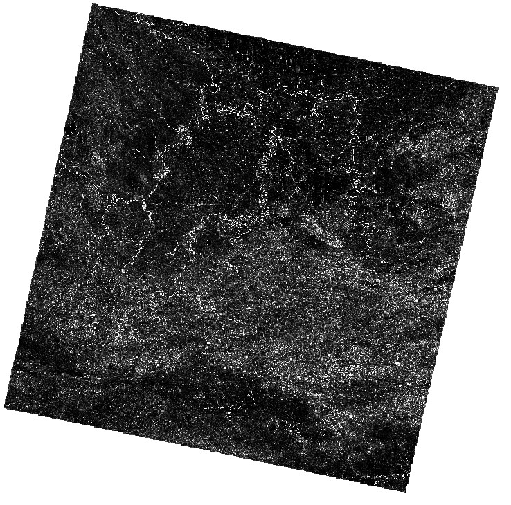
Image Sharpening#
All Landsat 8 bands are at approximately 30 m resolution, except for Band 8 (Panchromatic), which is at approximately 15 m resolution. The higher resolution Band 8 can be used to sharpen the imagery of the other bands. Pansharpening is typically done on three-band composites (see above). Each of these three bands is typically pansharpened separately and then combined into a new composite. The following formulae apply to an RGB composite (4-3-2), but any three bands can be used. Raster Calculator can be used to generate the pansharpened bands; be sure to specify the output resolution to be the same value as the panchromatic band (in this case 15 meters).
The Brovey Transformation
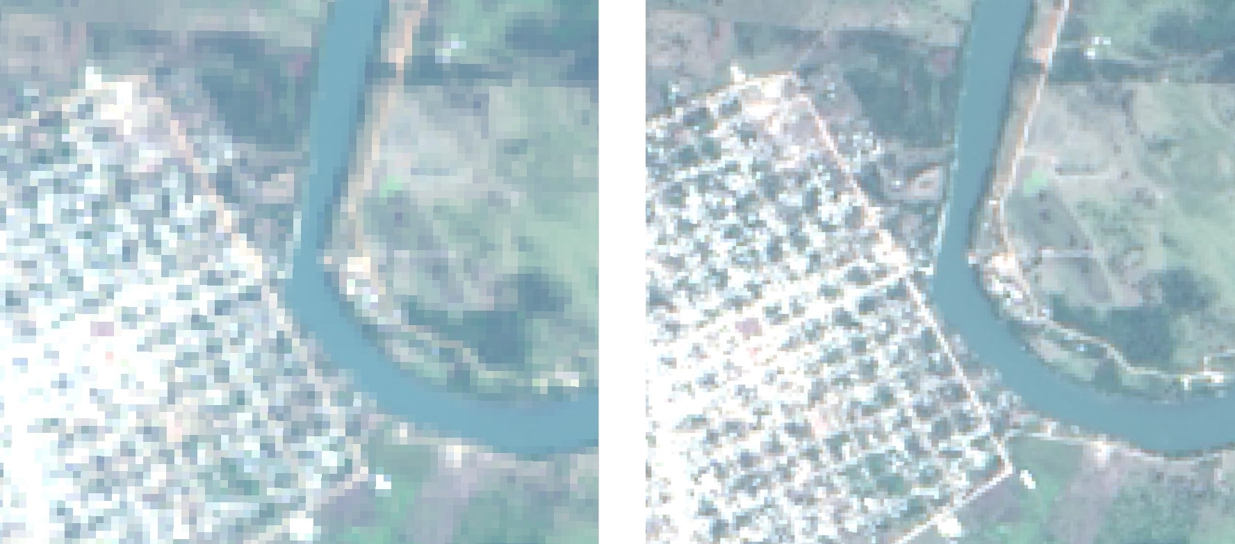
The new bands can then be combined into a new, pansharpened composite. The following images compare the original 30 meter RGB composite (left) with the pansharpened 15 meter RGB composite (right):
Simple Mean Transformation
Additional Transformations
Other transformations include Principal Components Analysis (PCA) pansharpening; Intensity, Hue, and saturation (IHS) pansharpening; and Gram-Schmidt pansharpening. These techniques are available in ArcGIS Pro’s Create Pansharpened Raster Dataset tool and in the QGIS/GRASS i.pansharpen tool.
Creating a Final Composite#
Multiple bands (including any of the original bands and derivatives) can be combined into a new multiband image. Theoretically, an infinite number of bands could be combined into a composite, but researchers should select the most useful bands for their application. Although the human eye can only view 3 bands at once (with perhaps a 4th alpha channel), classification algorithms can easily work with multidimensional data.
In ArcGIS Pro, the Composite Bands tool can combine several bands into a single file. In QGIS (GRASS), the r.composite tool can be used to combine only 3 bands, or bands can be combined into a virtual raster.
Building the following composite, we will use the following variables:
PCA1, PCA2, PCA3 refer to the 1st, 2nd, and 3rd order of the Principal Components Analysis, respectively.
vis – composite of visible bands (4, 3, 2)
ir – composite of infrared bands (7, 6, 5)
sb – San Bartolo composite of near infrared, green, and blue (5, 3, 2)
Var – texture variance index, 3 x 3 neighborhood
NDVI – Normalized Difference Vegetation Index
Chowdhury and Schneider (2004) recommended for southern Yucatan a 7-band composite: PCA1(vis), PCA1 (ir), PCA2 (ir), Var(PCA1(vis)), Var(PCA1(ir)), Var(PCA2(ir)), NDVI
Griffin (2012) recommended for Petén a 3-band composite: PCA1(sb), Var(PCA1(sb)), NDVI.
Using Griffin (2012)’s recommendation, we generate the following results:
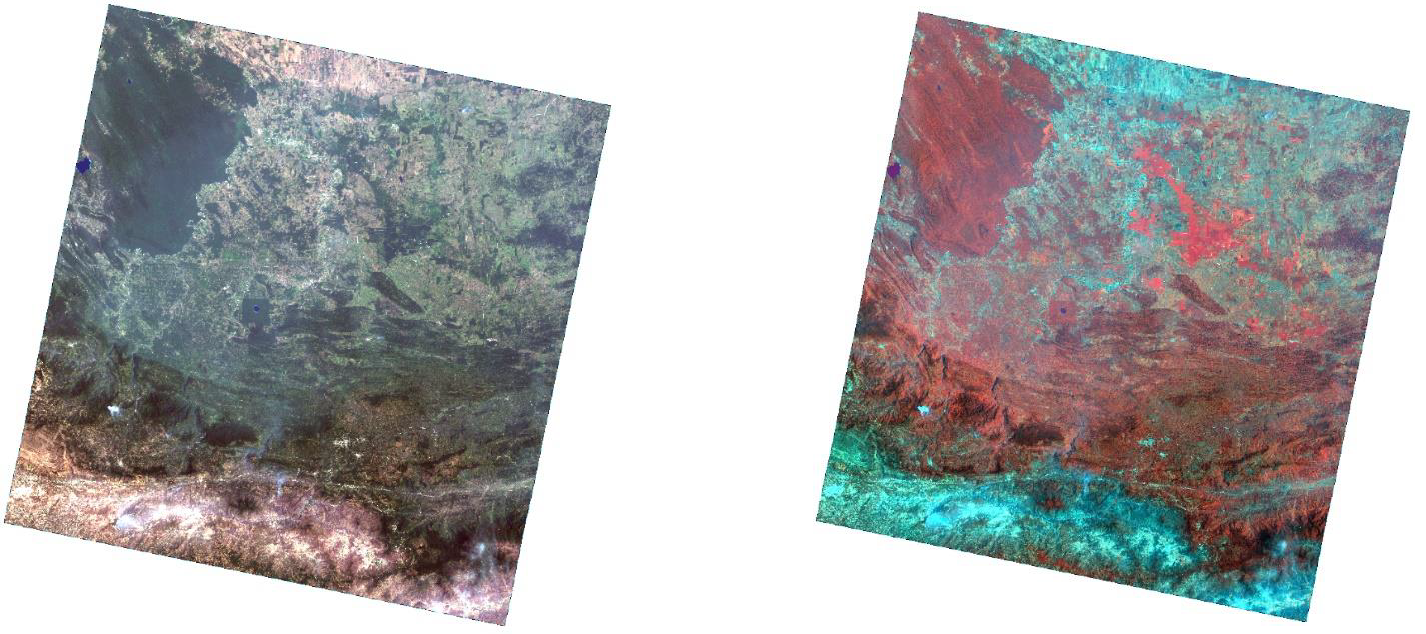
True Color RGB (left) and 5-3-2 composite (right), Southeastern Chiapas, Mexico
4/3/17, 16:23:16 Landsat 8,
CORNER_UL_LAT = 16.95093
CORNER_UL_LON = -91.54527
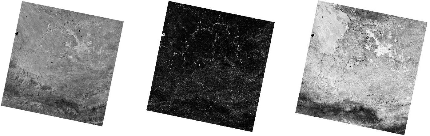
First order Principle Components Analysis of 5-3-2 composite (left), Textural variance of PCA1 (center), NDVI (right)
Preliminary interpretation:
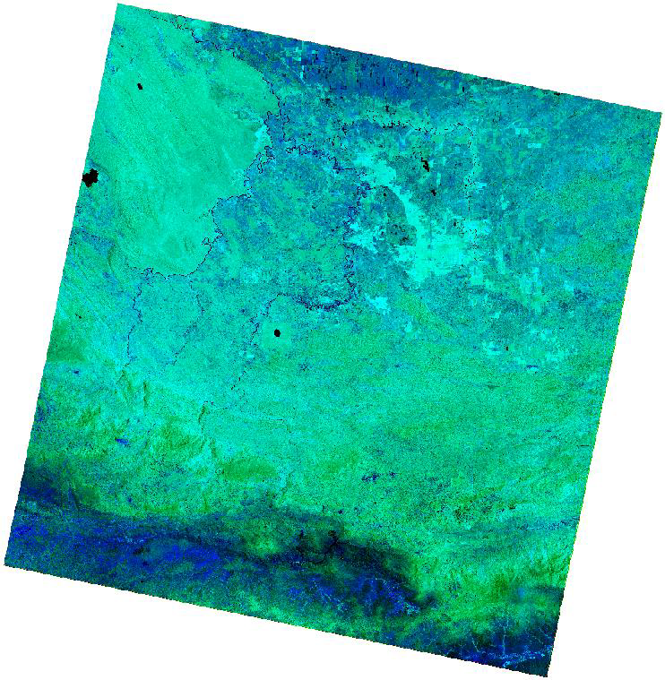
Final composite: Var (red)-NDVI (green)-PCA1 (blue)
Green – vegetation
Light green – healthy vegetation
Dark green – recently burned areas
Greenish white – lower vegetation
Whitish green – agriculture
Greenish brown – murky water Blue – water, urban, and bare earth
Dark blue – water
Bright blue – sandy beaches
Blue to magenta – exposed bedrock
Various shades of blue – urban and land use Red – shorelines and immediate land use changes
Planet Imagery#
Higher resolution (approximately 3-meter) multispectral satellite imagery is available at https://www.planet.com. Limited access to imagery (3,000 square kilometers per month download limit) is available for education and research: https://www.planet.com/industries/education-and-research/. To apply for the basic account, you will need to provide a .edu email address, personal information, and a brief description of your project. You should receive a verification email within a couple of weeks. Once your account is confirmed, you can login and access data through the Planet Explorer or Basemaps Viewer.
Aerial imagery in the visible range (red, green, and blue) can be downloaded from the Basemaps Viewer, which provides the highest quality cloud-free imagery available each month. Zoom into your area of interest, choose the layer of interest, and click View Quads and Scenes. Select a point or draw an area, then click Download Quad. Multispectral data is available in the Planet Explorer. In the Planet Explorer, zoom to your area of interest, and click the Draw or upload an area of interest button on the right. Choose an option to draw an area of interest. The menu on the left will populate with options. View imagery by clicking the eye icon in the top right of the imagery thumbnail. Once you’ve identified the appropriate imagery, add the items to your order, click Order Scenes, and click through the options. When ready, a download link will be emailed to your email address on file.
The downloaded imagery contains a raster showing the clipped region (imagery extent), and the multispectral imagery (usually containing AnalyticMS). Multispectral imagery contains 4 bands: near infrared (band 4), red (band 3), green (band 2), blue (band 1), or 8 bands: near infrared (band 8), red edge (band 7), red (band 6), yellow (band 5), green (band 4), green ii (band 3), blue (band 2), coastal blue (band 1). These bands can be visualized in QGIS or ArcGIS Pro with different band combinations, or they can be used to generate indices, such as the NDVI, texture analysis, or principal component analysis.
Readings#
Davis, D. S., Domic, A. I., Manahira, G., & Douglass, K. 2024. Geophysics Elucidate Long-term Socio-ecological Dynamics of Foraging, Pastoralism, and Mixed Subsistence Strategies on SW Madagascar. Journal of Anthropological Archaeology 75(101612). https://doi.org/10.1016/j.jaa.2024.101612
Estanqueiro, Marta, Aleksandar Šalamon, Helen Lewis, Barry Molloy, and Dragan Jovanović. 2023. Sentinel-2 Imagery Analyses for Archaeological Site Detection: An Application to Late Bronze Age Settlements in Serbian Banat, Southern Carpathian Basin. Journal of Archaeological Science: Reports 51:104188. https://doi.org/10.1016/j.jasrep.2023.104188
Ronchi, Diego, Marco Limongiello, Emanuel Demetrescu, and Daniele Ferdani. 2023. Multispectral UAV data and GPR survey for archeological anomaly detection supporting 3D reconstruction. Sensors 23:2769. https://doi.org/10.3390/s23052769
Alders, W., Davis, D.S. & Haines, J.J. 2024. Archaeology in the Fourth Dimension: Studying Landscapes with Multitemporal PlanetScope Satellite Data. Journal of Archaeological Method and Theory 31:1588–1621. https://doi.org/10.1007/s10816-024-09644-x.
Brondizio and Chowdhury. 2010. Spatiotemporal methodologies in environmental anthropology: geographic information systems, remote sensing, landscape changes, and local knowledge. In: Vaccaro I, Smith EA, Aswani S, eds. Environmental Social Sciences: Methods and Research Design. Cambridge University Press, pp. 266-298.
Garrison, Thomas G., Stephen D. Houston, Charles Golden, Takeshi Inomata, Zachary Nelson, and Jessica Munson. 2008. Evaluating the Use of IKONOS Satellite Imagery in Lowland Maya Settlement Archaeology. Journal of Archaeological Science 35(10):2770-2777. https://doi.org/10.1016/j.jas.2008.05.003
Additional References#
Parcak, Sarah. 2009. Satellite Remote Sensing for Archaeology. Routledge, New York.
Amidon, Will. Middlebury Remote Sensing. https://www.youtube.com/channel/UCgNXU17K63E2fzWxYv1-_4w/featured
Chowdhury, Rinku Roy, and Laura Schneider. 2004. Land Cover and Land Use: Classification and Change Analysis. In Integrated Land-Change Science and Tropical Deforestation in the Southern Yucatan: Final Frontiers, ed. B.L. Turner II, Jacqueline Geoghegan, and David R. Foster, 105–143. Oxford: Oxford University Press. https://doi.org/10.1093/oso/9780199245307.003.0015
Griffin, Robert Edward. 2012. The Carrying Capacity of Ancient Maya Swidden Maize Cultivation: A Case Study in the Region Around San Bartolo, Petén, Guatemala. Unpublished PhD dissertation, Pennsylvania State University. https://etda.libraries.psu.edu/catalog/15390
Saturno, William, Thomas L. Sever, Daniel E. Irwin, Burgess F. Howell, and Thomas G. Garrison. 2007. Putting Us on the Map: Remote Sensing Investigation of the Ancient Maya Landscape. In Remote Sensing in Archaeology, edited by James Wiseman and Farouk El-Baz, pp. 137-160. Springer, New York. https://link.springer.com/chapter/10.1007/0-387-44455-6_6