8. Visualizing and Processing Lidar Point Clouds in R with the lidR Package#
In this lab, students will learn how to load, visualize, and process lidar point clouds in R. Before proceeding, download the latest versions of R and R Studio at the following link: https://posit.co/download/rstudio-desktop.
Processing lidar in R has several advantages, namely that it is free and open source. The drawback is that as a programming language, R is generally slower than others including Python and C++.
Install and load libraries#
If you are not familiar with R, after downloading, open R Studio and install the following libraries or packages:
# The lidR package is used for processing las point clouds

install.packages("lidR", dependencies = TRUE)

# The following packages are used for several remote sensing
# applications and for generating raster surfaces

install.packages("RStoolbox")
install.packages("terra")
install.packages("raster")

# ggplot is used to produce publication quality images
install.packages("ggplot2")

# RColorBrewer loads several useful color palettes for data visualization
install.packages("RColorBrewer")
Note
You only have to use the install.packages command once. After all packages are installed, you will just have to load the necessary libraries every time you run the code.
If you see a warning that Rtools is not installed, download the appropriate version of Rtools for your R version here.
To get your R version, run the following in RStudio:
version
Once installed, run the following to load the libraries:
library(lidR)
library(RStoolbox)
library(terra)
library(raster)
library(ggplot2)
library(RColorBrewer)
Download and import data#
lidR is a point cloud oriented software, so we first have to download a point cloud in either .las or .laz format.
In this lab, we will use publicly available data from the NASA G-LiHT system. Data can be browsed at https://glihtdata.gsfc.nasa.gov/files/G-LiHT. For this exercise, download the AMIGACarb_Yuc_Centro_GLAS_Apr2013_l1s460.las.gz file. You will need 7-zip to extract the .las file.
Now, import the file into R. You can either copy the folder path and load into R, or copy the file to your working directory. To determine your working directory:
getwd()
Or to change your working directory:
setwd("C:\\Your\\Full\\Directory\\Here")
Assuming your file is in your working directory:
# Import file
# Creates a string based on your file location

file <- "AMIGACarb_Yuc_Centro_GLAS_Apr2013_l1s460.las"

# Reads the file as an .las or .laz

las <- readLAS(file)
We can summarize the .las statistics with the following code:
# Summarize las statistics
# Provides the header of the .las file

print(las)
class : LAS (v1.1 format 1)
memory : 2.8 Gb
extent : 277008.5, 278391.3, 2070914, 2079175 (xmin, xmax, ymin, ymax)
coord. ref. : WGS 84 / UTM zone 16N
area : 3.22 km²
points : 50.99 million points
density : 15.84 points/m²
density : 10.43 pulses/m²
# Provides the header of the .las file and additional information.

summary(las)

# Provides additional header information in tabular format

payload(las)

# Displays the number of points and their classification

table(las$Classification)

# Generates a histogram of the selected data

hist(las$Intensity)

hist(las$ReturnNumber)
1 2
30522821 20462312
The current American Society for Photogrammetry and Remote Sensing (ASPRS) standard classification codes for point data are:
Classification Value |
Meaning |
|---|---|
0 |
Created, never classified |
1 |
Unclassified |
2 |
Ground |
3 |
Low Vegetation |
4 |
Medium Vegetation |
5 |
High Vegetation |
6 |
Building |
7 |
Low Point (noise) |
8 |
Reserved |
9 |
Water |
10 |
Rail |
11 |
Road Surface |
12 |
Reserved |
13 |
Wire - Guard (Shield) |
14 |
Wire - Conductor (Phase) |
15 |
Transmission Tower |
16 |
Wire-structure Connector (e.g., Insulator) |
17 |
Bridge Deck |
18 |
High Noise |
19-63 |
Reserved |
64-255 |
User definable |
We can see that the point data have only been classified into Ground, which is usually fine for archaeology. Later, we can further classify the points into vegetation, noise, etc. This lab will focus on how to perform the initial classification into ground and non-ground points.
We can also filter the point cloud data, for example, if we only want to work with ground points. We can also load less data to aid in processing.
# Load only ground points (classified as 2) with only spatial x, y, z
# coordinates, classification (c), and return number (r)
lasground <- readLAS(file, filter = "-keep_class 2", select = "xyzcr")

# Displays all filter options
readLAS(filter = "-help")
Attribute abbreviations for the select option:
x |
x coordinates of points |
y |
y coordinates |
z |
z coordinates (in reality xyz are always loaded by default) |
c |
classification code |
r |
return number |
i |
intensity |
t |
gpstime |
a |
scan angle |
n |
number of returns |
s |
synthetic flag |
k |
keypoint flag |
w |
withheld flag |
o |
overlap flag |
u |
user data |
p |
point source id |
e |
edge of flight line flag |
d |
direction of scan flag |
R |
red channel (RGB) |
G |
green channel |
B |
blue channel |
N |
near-infrared channel |
C |
scanner channel |
W |
full waveform |
Now if we summarize just lasground, we get only the points we loaded with classification code 2.
print(lasground)

table(lasground$Classification)
class : LAS (v1.1 format 1)
memory : 546.4 Mb
extent : 277008.5, 278391.3, 2070914, 2079175 (xmin, xmax, ymin, ymax)
coord. ref. : WGS 84 / UTM zone 16N
area : 3.15 km²
points : 20.46 million points
density : 6.5 points/m²
density : 3.33 pulses/m²
2
20462312
The plot function displays point cloud data, but it is computationally intensive. I recommend viewing point clouds in dedicated software like Cloud Compare.
plot(lasground)

vox <- voxelize_points(lasground, 6)
plot(vox, voxel = TRUE, bg = "white")
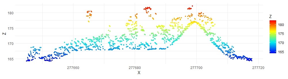
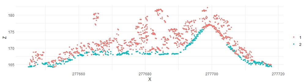
Jean-Romain Roussel, Tristan R.H. Goodbody, and Piotr Tompalski offer a useful function to plot cross sections of point data. Cross sections can be useful to view the accuracy of ground classification.
First, you will need to define the coordinates of your cross section. Using QGIS or Google Earth, identify coordinates p1 and p2 that are within your study area. The p1 variable defines the (x,y) coordinates of the first point, and the p2 variable defines the (x,y) coordinates of the second point. Connecting these two points creates your profile line.
# Define the x and y coordinates for the cross section, and the width of the
# cross section.

p1 <- c(277645, 2074590)
p2 <- c(277718, 2074681)
width <- 1

# Define the plot_crossection function

plot_crossection <- function(las, p1, p2, width, colour_by = NULL) {
  colour_by <- rlang::enquo(colour_by)
  data_clip <- clip_transect(las, p1, p2, width)
  p <- ggplot(data_clip@data, aes(X,Z)) + geom_point(size = 0.5) + coord_equal() + theme_minimal()

  if (!is.null(colour_by))
    p <- p + aes(color = !!colour_by) + labs(color = "")

  return(p)
}

# Plot the crossection by elevation

data_clip <- clip_transect(las, p1, p2, width)

ggplot(data_clip@data, aes(X,Z, color = Z)) +
  geom_point(size = 0.5) +
  coord_equal() +
  theme_minimal() +
  scale_color_gradientn(colours = height.colors(50))
# Plot the crossection by classification
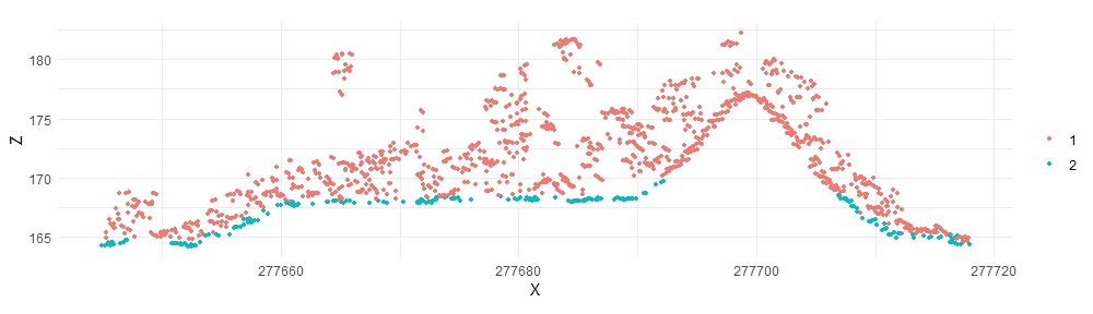
plot_crossection(las, p1, p2, width, colour_by = factor(Classification))
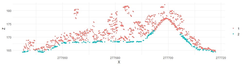
Based on this crossection, the ground classification failed in some areas. We’ll pursue options later to improve the ground classification in R.
If you get an error message in this step, it is likely due to your p1 and p2 points being incorrect. You can plot your cross section line over a raster of your data to verify the points line up with your data. See below under the plot density function.
Generate Raster Surfaces#
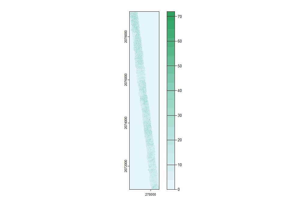
Several raster surfaces can be generated from point cloud data, including but not limited to digital elevation models. For example, we can get a sense of the distribution of points across the dataset by plotting the density of returns. Use R Color Brewer for additional color palettes.
# Generate the density grid; res refers to the resolution or cell size of the resulting
# surface. In this example, the resulting surface will show the number of points per
# square meter.

density <- rasterize_density(las, res=1)

# Specify the color palette

cols <- brewer.pal(9, "BuGn")
pal <- colorRampPalette(cols)

# Plot density

plot(density, col = pal(20))
To visualize your profile line based on variables p1 and p2 above, after plotting the density raster, run the following:
segments(x0 = p1[1], y0 = p1[2], x1 = p2[1], y1 = p2[2], col = "black", lwd = 5, lty = "dotted")
You should see the profile line plotted over the raster. If you do not see your profile line, your points are outside of the data. You will have to determine correct values and redefine the p1 and p2 variables above.
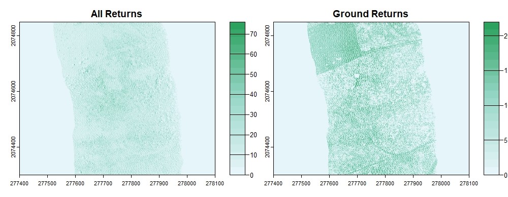
We can also generate a density surface using only ground classified points, and we can set the axis limits to better view the data.
densitygr <- rasterize_density(lasground, res=1)

plot(density, maxcell = Inf, xlim = c(277400, 278100), ylim = c(2074300, 2074850), col=pal(20))
plot(densitygr, maxcell = Inf, xlim = c(277400, 278100), ylim = c(2074300, 2074850), col=pal(20))
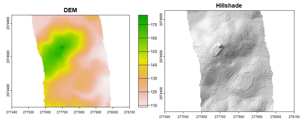
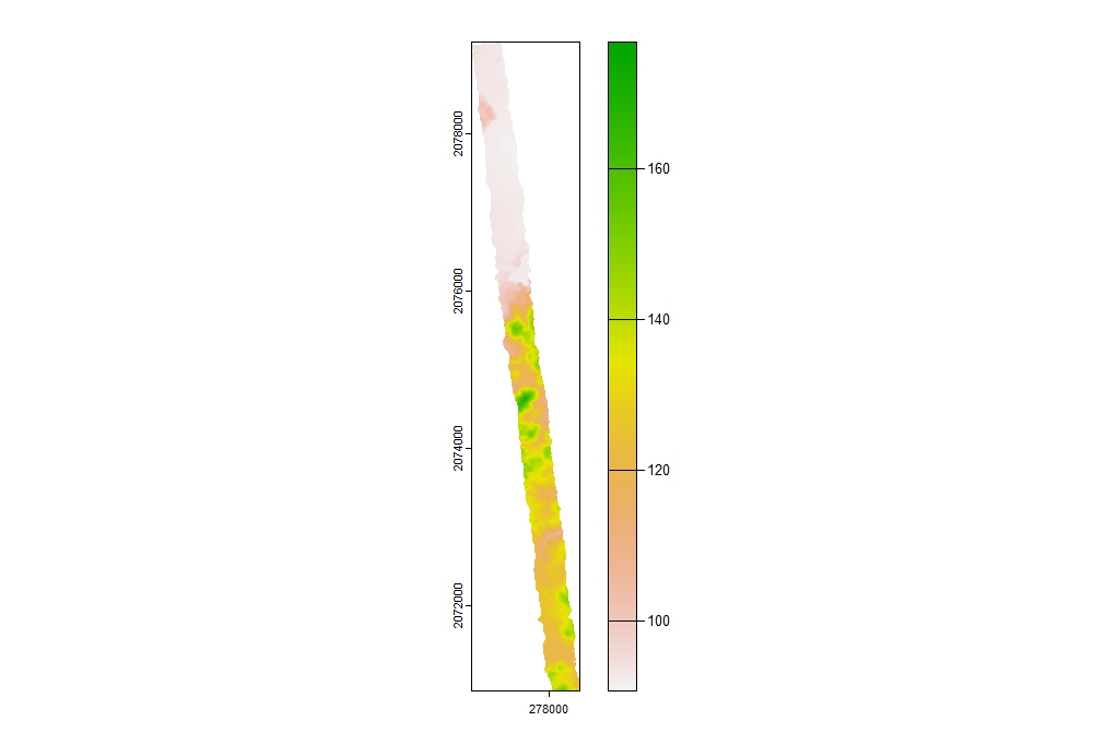
Generate Digital Elevation Model#
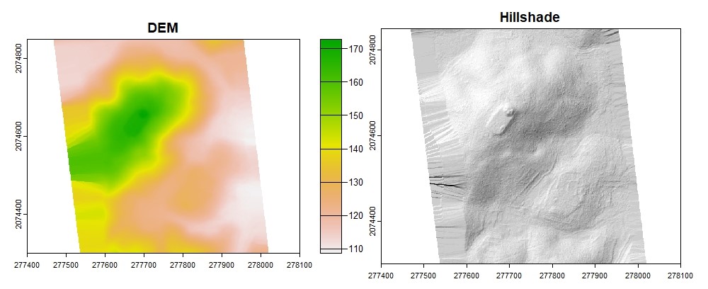
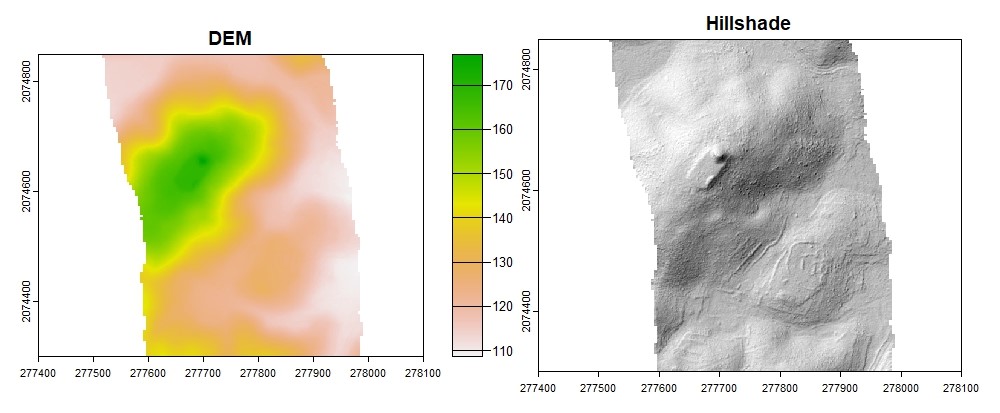
The lidR package has several interpolation algorithms. We will use Invert Distance Weighting because it is a relatively simple algorithm with acceptable results.
#DEM

dtm_idw <- rasterize_terrain(las, res = 1, algorithm = knnidw(k = 10L, p = 2))
terrcols <- brewer.pal(11, "RdYlGn")
plot(dtm_idw, col = rev(terrcols), maxcell = Inf, xlim = c(277400, 278100), ylim = c(2074300, 2074850))

#Hillshade

dtm_prod <- terrain(dtm_idw, v = c("slope", "aspect"), unit = "radians")
dtm_hillshade <- shade(slope = dtm_prod$slope, aspect = dtm_prod$aspect, angle = 45, direction = 315)
plot(dtm_hillshade, col = gray(0:30/30), maxcell = Inf, legend = FALSE, xlim = c(277400, 278100), ylim = c(2074300, 2074850))
For a more continuous DEM:
plot(dtm_idw, col = terrain.colors(100), maxcell = Inf, xlim = c(277400, 278100), ylim = c(2074300, 2074850))
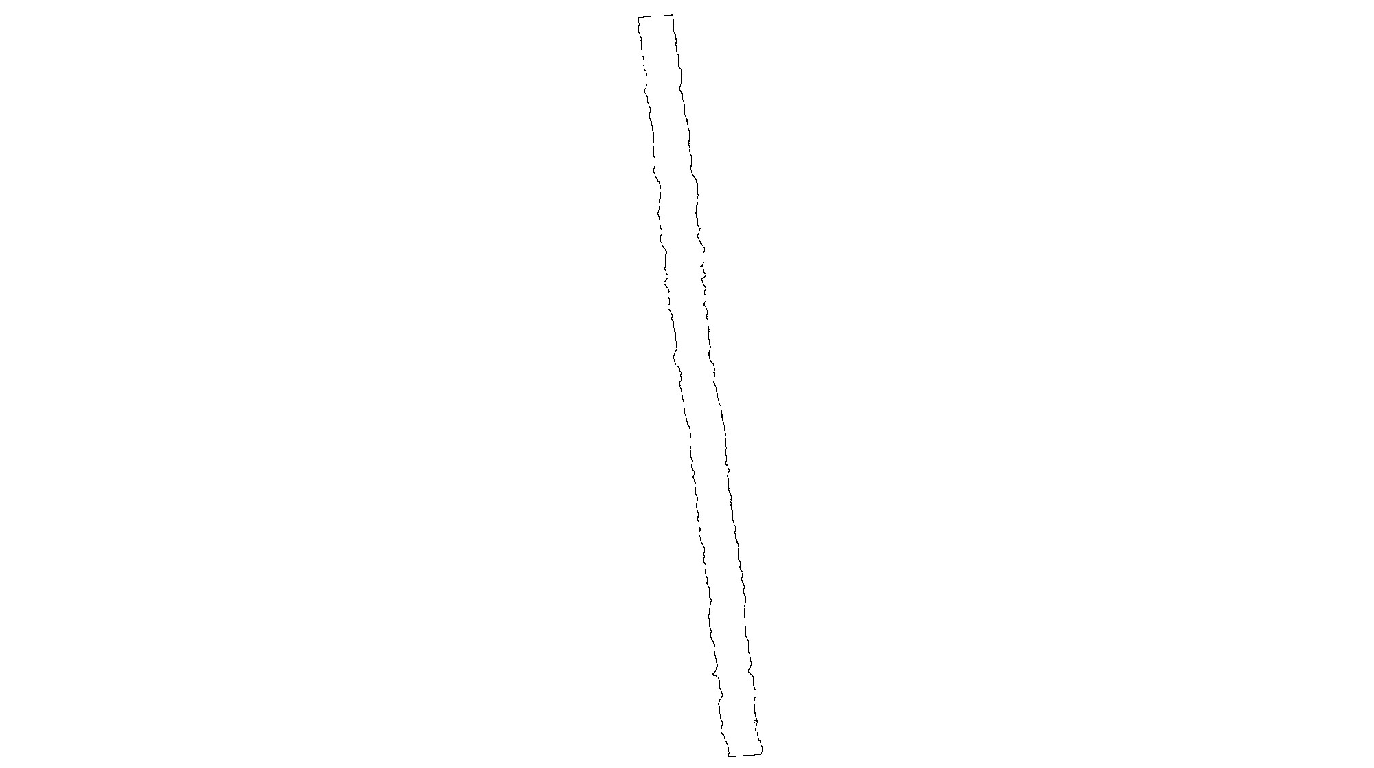
An issue with the default convex hull method of interpolation is that it interpolates too much of the edges of irregular point cloud extents. Using the concave hull option can be an improvement but better results are possible using a polygon based on the density surface extent to force proper edges. This step is not necessary for more uniform extents.
# Generate a new density surface with a coarser resolution. Not every square meter has
# a return. Choose a value that will ensure continuous data with no gaps.

density <- rasterize_density(las, res=5)

# Convert density surface to raster

dens <- raster(density)

# Reclassify density (slice into single value) and convert to polygon

reclass <- c(0, Inf, 1)
reclass_m <- matrix(reclass, ncol = 3, byrow = TRUE)
densreclass <- reclassify(dens, reclass_m)
densreclass[densreclass == 0] <- NA
densreclasssr <- as(densreclass, "SpatRaster")
lasspvect <- as.polygons(densreclasssr)
lassf <- sf::st_as_sf(lasspvect)
lassfc <- sf::st_as_sfc(lassf)

plot(lassfc)
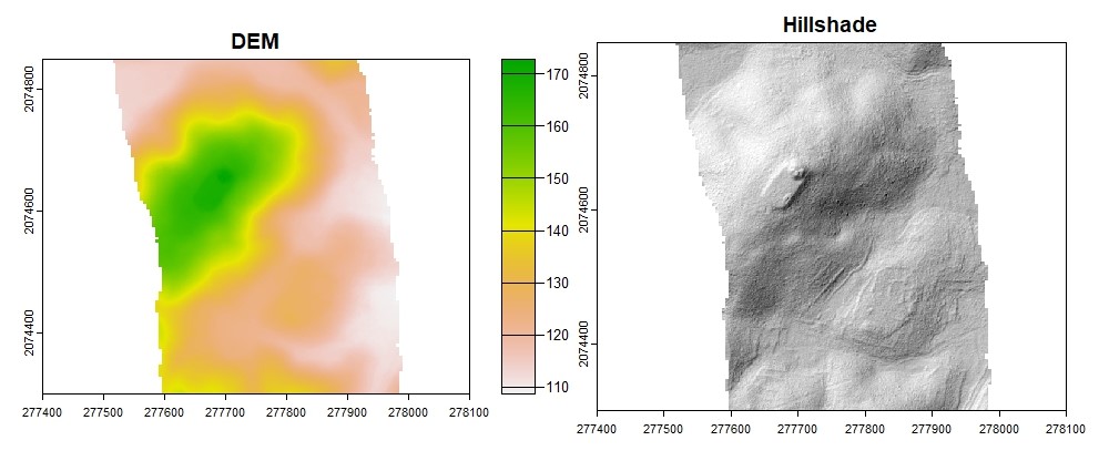
We now have an outline of the point cloud extent that we can use in the interpolation as a shapefile.
dtm_idw <- rasterize_terrain(las, res = 1, algorithm = knnidw(k = 10L, p = 2),
		shape = lassfc)
plot(dtm_idw, col = rev(terrcols), maxcell = Inf, xlim = c(277400, 278100), ylim = c(2074300, 2074850))

#Hillshade

dtm_prod <- terrain(dtm_idw, v = c("slope", "aspect"), unit = "radians")
dtm_hillshade <- shade(slope = dtm_prod$slope, aspect = dtm_prod$aspect, angle = 45, direction = 315)
plot(dtm_hillshade, col = gray(0:30/30), maxcell = Inf, legend = FALSE, xlim = c(277400, 278100), ylim = c(2074300, 2074850))
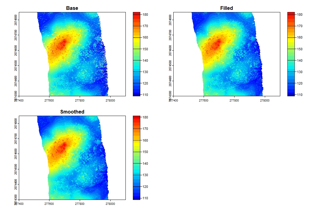
Generate Digital Surface Model#
The digital surface model is a raster where each cell represents the highest elevation of returns. When generated from elevation (Z) data, the raster is a digital surface model. When generated from a normalized point cloud (height above ground), the raster is a canopy height model.
# Standard DSM

dsm <- rasterize_canopy(las, res = 1, algorithm = p2r())
col <- height.colors(25)

# DSM using circles with 0.15 m radius to fill gaps

dsm <- rasterize_canopy(las, res = 0.5, algorithm = p2r(subcircle = 0.15), pkg = "terra")

# Filled DSM

fill.na <- function(x, i=5) { if (is.na(x)[i]) { return(mean(x, na.rm = TRUE)) } else { return(x[i]) }}
w <- matrix(1, 3, 3)

filled <- terra::focal(dsm, w, fun = fill.na)

# Smoothed DSM

smoothed <- terra::focal(dsm, w, fun = mean, na.rm = TRUE)

dsms <- c(dsm, filled, smoothed)
names(dsms) <- c("Base", "Filled", "Smoothed")
plot(dsms, col = col, maxcell = Inf, xlim = c(277400, 278100), ylim = c(2074300, 2074850))
Ground classification#
Although the point cloud was already classified into ground points, we have seen that the ground classification could be improved. Ground classification is computationally intensive, so we have to first retile the point cloud into more manageable, smaller chunks. To do this we will reload the point cloud as an las catalog.
lascat <- readLAScatalog(file)

# Set a location to retile into smaller .las files, create a 25 m buffer around tiles,
# and set the tile size to 1600 x 1600 m

opt_output_files(lascat) <- "C:/AMIGACarb_Yuc_Centro_GLAS_Apr2013 processed BE/Point Clouds/s460{XLEFT}_{YBOTTOM}"
opt_chunk_buffer(lascat) <- 25
opt_chunk_size(lascat) <- 1600
small <- catalog_retile(lascat)
R has 3 built-in ground classification algorithms, Cloth Simulation Function, Progressive Morphological Filter, and Multiscale Curvature Classification. Refer to Štular and Lozić (2020) for recommendations for parameters.
To experiment with ground classification algorithms, it is best to load a smaller dataset; for example, one of the tiles we created in the last step.
lastest <- readLAS("C:/AMIGACarb_Yuc_Centro_GLAS_Apr2013 processed BE/Point Clouds/s460276800_2073600.las")
Cloth Simulation Function (CSF)#
The CSF algorithm models the ground surface by first flipping the point cloud upside down and imagining draping a cloth over the points. Based on different paramaters representing the rigidity of the cloth, the resolution or point spacing, and the force of gravity or weight of the cloth, the function creates a surface over the points that is then flipped back over to model the ground.
The CSF algorithm is advantageous because it is relatively fast. However, the results are error prone, with many points misclassified. The CSF algorithm is best used to quickly assess terrain models or to generate DEMs with coarser resolutions, especially if the end goal is modeling vegetation above ground.
We will start with the default parameters.
mycsf <- csf(sloop_smooth = FALSE, class_threshold = 0.5, cloth_resolution = 0.5, rigidness = 1, iterations = 500L, time_step = .65)
lascsf <- classify_ground(lastest, mycsf)
# Plot the new classification
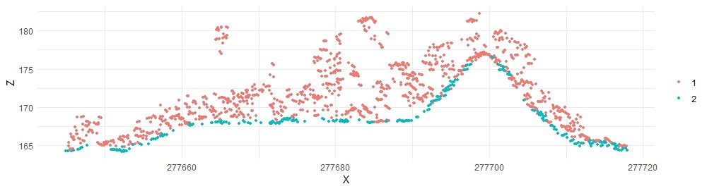
plot_crossection(lascsf, p1, p2, width, colour_by = factor(Classification))
The large mound is still not correctly classified. We can try different parameters:
mycsf <- csf(sloop_smooth = TRUE, class_threshold = 0.3, cloth_resolution = 0.5, rigidness = 1, iterations = 1000L, time_step = .75)
lascsf2 <- classify_ground(lastest, mycsf)
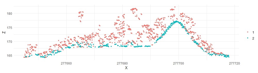
The results are improved on top of the mound, but now many of the ground points in flat areas are misclassified, leading to a noisey DEM. We can keep trying different parameters or use a different algorithm.
Progressive Morphological Filter#
The PMF algorithm uses a moving window to classify points as ground within a certain threshold of neighboring points. The filter is progressive because sequences of window sizes and thresholds are applied to the point cloud. The window size generally begins with a smaller size (in the units of the point cloud), then a larger size, then a final step with the original smaller size. The threshold generally increases from a smaller to a larger value, either linearly or exponentially. Exponentially is recommended because processing time is significantly reduced.
The PMF algorithm has the potential to be highly accurate; however, the drawback is that processing time is much higher, and nearly an infinite number of parameters are available for experimentation, making it difficult to refine settings.
We will begin with the recommended parameters in Štular and Lozić (2020).
ws <- seq(3, 12, 3)
th <- seq(0.3, 1.5, length.out = length(ws))
laspmf <- classify_ground(lastest, algorithm = pmf(ws = ws, th = th))

plot_crossection(laspmf, p1, p2, width, colour_by = factor(Classification))
These results, in fact, look very similar to the already classified points provided in the original NASA G-LiHT dataset. Although Štular and Lozić observed that decreasing the window size had no noticeable impact on results, I have found that for archaeological features, smaller window sizes are necessary. VanValkenburgh and colleagues (2020) used window sizes as low as 0.6 m.
ws <- seq(1, 8, 1)
th <- seq(0.1, 1, length.out = length(ws))
laspmf2 <- classify_ground(lastest, algorithm = pmf(ws = ws, th = th))

plot_crossection(laspmf2, p1, p2, width, colour_by = factor(Classification))
The ground classification is significantly improved.
Multiscale Curvature Classification#
The MCC algorithm uses deviations from positive curvature thresholds to progressively eliminate non-ground points. The following default values lead to acceptable results:
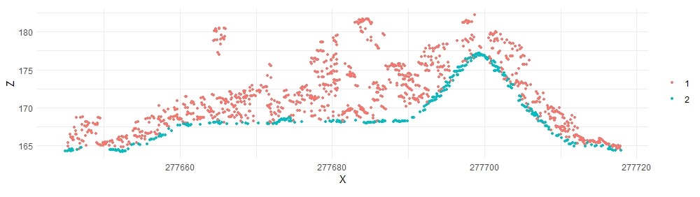
lasmcc <- classify_ground(lastest, mcc(1.5,0.3))

plot_crossection(lasmcc, p1, p2, width, colour_by = factor(Classification))
With minor tweaking, we can get even better results:
lasmcc2 <- classify_ground(lastest, mcc(1,0.3))

plot_crossection(lasmcc2, p1, p2, width, colour_by = factor(Classification))


Classifying all tiles with lascatalog#
We can now apply what we determine to be the most appropriate algorithm and parameters to the entire dataset using lascatalog. Let’s set up our lascatalog again.
lascat <- readLAScatalog(file)
Alternatively, you can load a set of .las files from a folder:
lascat <- readLAScatalog("C:/AMIGACarb_Yuc_Centro_GLAS_Apr2013 processed BE/Point Clouds/")
Set the same tile size and buffer as before with new output files in a different folder. Then apply the MCC algorithm and parameters to the full dataset.
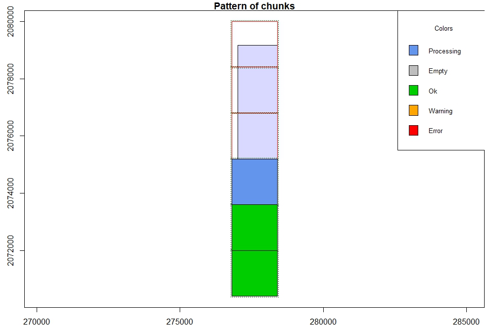
opt_chunk_size(lascat) <- 1600
opt_chunk_buffer(lascat) <- 25
plot(lascat, chunk_pattern = TRUE)
opt_output_files(lascat) <- "C:/AMIGACarb_Yuc_Centro_GLAS_Apr2013 processed BE/ground/s460{XLEFT}_{YBOTTOM}g"

lasmccall <- classify_ground(lascat, mcc(1, 0.3))
We can then process the DEM based on the new ground classification.
dtm_idw <- rasterize_terrain(lasmccall, res = 1, algorithm = knnidw(k = 10L, p = 2), shape = lassfc)

plot(dtm_idw)
Once you are satisfied with the ground classification, you can output results as a raster.
writeRaster(dtm_idw, "C:/AMIGACarb_Yuc_Centro_GLAS_Apr2013 processed BE/s460gr.tif")
Readings#
Fernandez-Diaz, Juan Carlos, William E. Carter, Ramesh L. Shrestha, and Craig L. Glennie. 2014. Now You See It… Now You Don’t: Understanding Airborne Mapping LiDAR Collection and Data Product Generation for Archaeological Research in Mesoamerica. Remote Sensing 6(10):9951–10001. https://doi.org/10.3390/rs6109951
Rostain, Stephén, Antoine Dorison, Geoffrey de Saulieu, Heiko Prümers, Jean-Luc le Pennec, Fernando Mejía Mejía, Ana Maritza Freire, Jaime R. Pagán-Jiménez, and Philippe Descola. 2024. Two Thousand Years of Garden Urbanism in the Upper Amazon. Science 383(6679). https://doi.org/10.1126/science.adi6317
Štular, Benjamin and Edisa Lozić. 2020. Comparison of Filters for Archaeology-Specific Ground Extraction from Airborne LiDAR Point Clouds. Remote Sensing 12(18):3025. https://doi.org/10.3390/rs12183025
VanValkenburgh, Parker, K.C. Cushman, Luis Jaime Castillo Butters, Carol Rojas Vega, Carson B. Roberts, Charles Kepler, and James Kellner. 2020. Lasers without lost cities: using drone lidar to capture architectural complexity at Kuelap, Amazonas, Peru. https://doi.org/10.1080/00934690.2020.1713287
Additional References#
Mohan, Midhun, Rodrigo Vieira Leite, Eben North Broadbent, et al. 2021 (forthcoming). Individual Tree Detection Using UAV-lidar and UAV-SfM Data: A Tutorial for Beginners. Remote Sensing 12.
Roussel, Jean-Romain, Tristan R.H. Goodbody, and Piotr Tompalski. 2023. The lidR package. https://r-lidar.github.io/lidRbook/index.html
VanValkenburgh, Parker. 2023. Seeing Through Trees: Lidar, Archaeology and the Possibility of Seeing Otherwise. In Active Landscape Photography, edited by Anne C. Godfrey. Routledge, London. https://www.taylorfrancis.com/chapters/edit/10.4324/9781003087717-5/seeing-trees-parker-vanvalkenburgh
Young, James. LiDAR for Dummies. <https://ibis.geog.ubc.ca/courses/geog373/lectures/ Handouts/LiDARforDummies.pdf>