9. Ground Penetrating Radar#
We will be using the RGPR package in R to plot GPR data. After installing R and RStudio, install and load RGPR and its dependencies.
# install "devtools" if not already done
if(!require("devtools")) install.packages("devtools")
devtools::install_github("emanuelhuber/RGPR")
# load RGPR in the current R session
library(RGPR)
Reitz Field#
Download the Reitz Field data to your working directory. You can determine your working directory by running the following:
getwd()
Or you can set your working directory:
setwd("C:\\Your\\Working\\Directory")
Once your data are in your working directory, run the following to change your working directory to the subfolder REITZ.PRJ:
setwd("./REITZ.PRJ")
The REITZ.PRJ folder should have all of the .dzt files, each one representing a single transect.
Now load the Reitz data from the directory and make sure that after running print(LINES), you can see a list of all your files with the correct folder structure:
LINES <- file.path(getwd(), paste0("REITZ_", sprintf("%04d", 1:11), ".DZT"))

print(LINES)
The code searches the working directory folder (in this case REITZ.PRJ) and loads all files ending in .dzt, beginning with REITZ_, followed by a 4 digit number ending in 1 through 11. This code will have to be updated depending on how the files are stored.
Next we load the lines and define their orientation:
mySurvey <- GPRsurvey(LINES)
# The next line of code creates 11 lines, separated by 0.5 m
# (negative indicates moving from left right), with a length of 15 m
setGridCoord(mySurvey) <- list(xlines = 1:11,
xpos = seq(0, by = -0.5, length.out = 11),
xstart = rep(0, 11),
xlength = rep(15, 11))
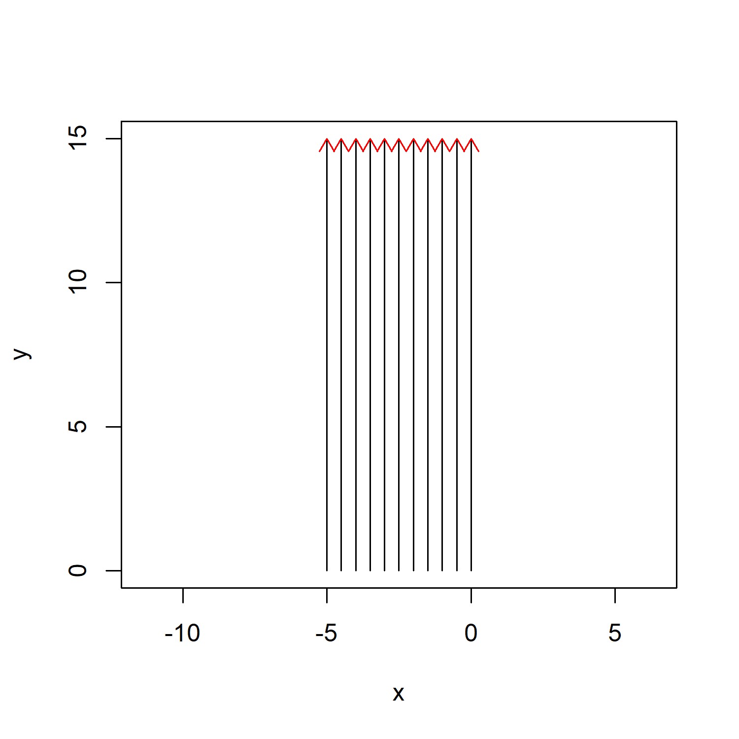
# Now we can plot the survey without fiduciary markers
plot(mySurvey, parFid = NULL)
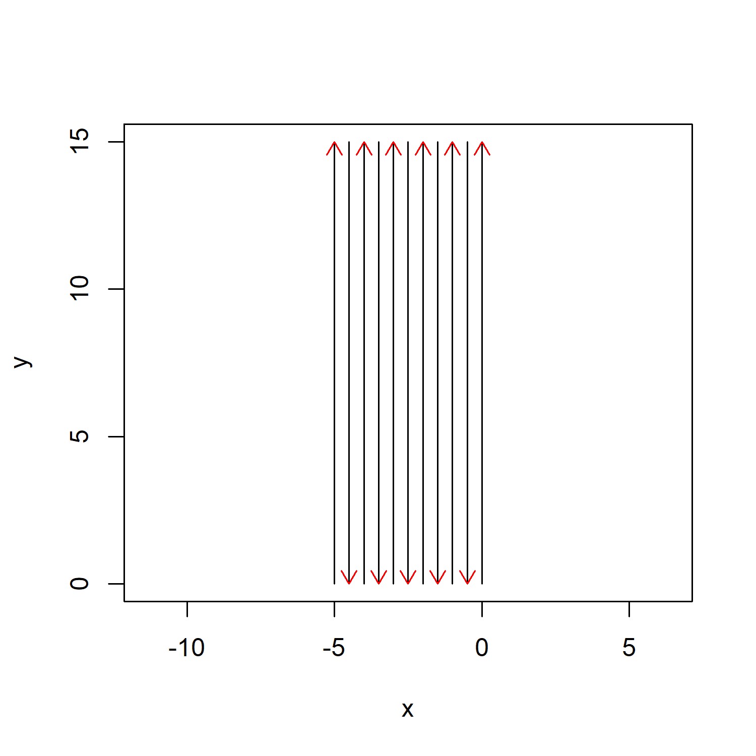
However, according to our notes, we alternated directions with each transect. Starting from the southeast ending at the northwest. The following code reverses every other transect:
mySurvey <- reverse(mySurvey, id = "zigzag")
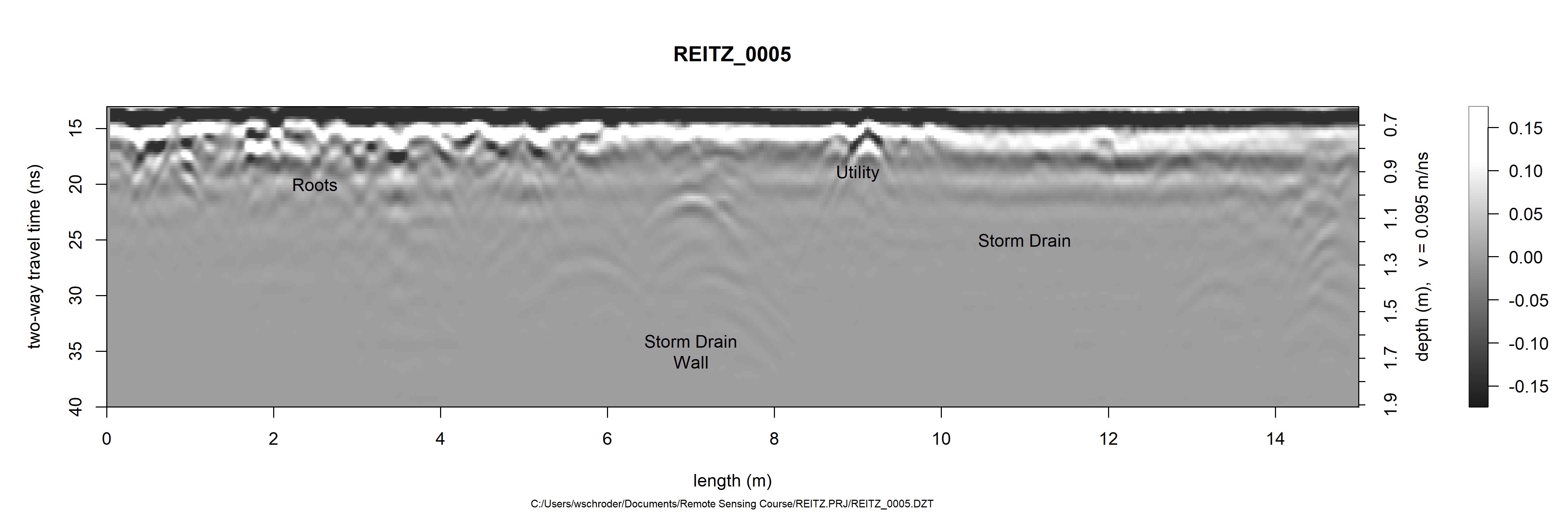
To plot the fifth profile (in order of data collection from right to left):
plot(mySurvey[[5]], relTime0 = TRUE, addFid = FALSE, col = palGPR("grey2"), ylim = c(13,40))
We can try to interpret some of the signals as shown:
Finally, we can interpolate the lines and plot a slice:
SXY <- interpSlices(mySurvey, dx = 0.15, dy = 0.15, dz = 0.56, h = 10)

plot(SXY[,,120], col = palGPR("grey2"))
There appears to be a storm drain running from northeast to the middle west, turning at a right angle to the southeast. However, more processing is needed to clarify.
Hollister Site#
Download the Hollister Site data to your working directory. You can determine your working directory by running the following:
getwd()
Once your data are in your working directory, run the following to change your working directory to the subfolder hollister_grid3:
setwd("./Hollister Site/hollister_grid3")
Now load the Hollister Site data from the directory and make sure that after running print(LINES), you can see a list of all your files with the correct folder structure:
LINES <- file.path(getwd(), paste0("FILE", sprintf("%03d", 101:181), ".DZT"))

print(LINES)
Next we load the lines and define their orientation:
mySurvey <- GPRsurvey(LINES)

# The next line of code creates 81 lines, separated by 0.5 m, with a length of 40 m

setGridCoord(mySurvey) <- list(xlines = 1:81,
                             xpos = seq(0, by = 0.5, length.out = 81),
                             xstart = rep(0, 81),
                             xlength = rep(40, 81))

# Now we can plot the survey without fiduciary markers

plot(mySurvey, parFid = NULL)
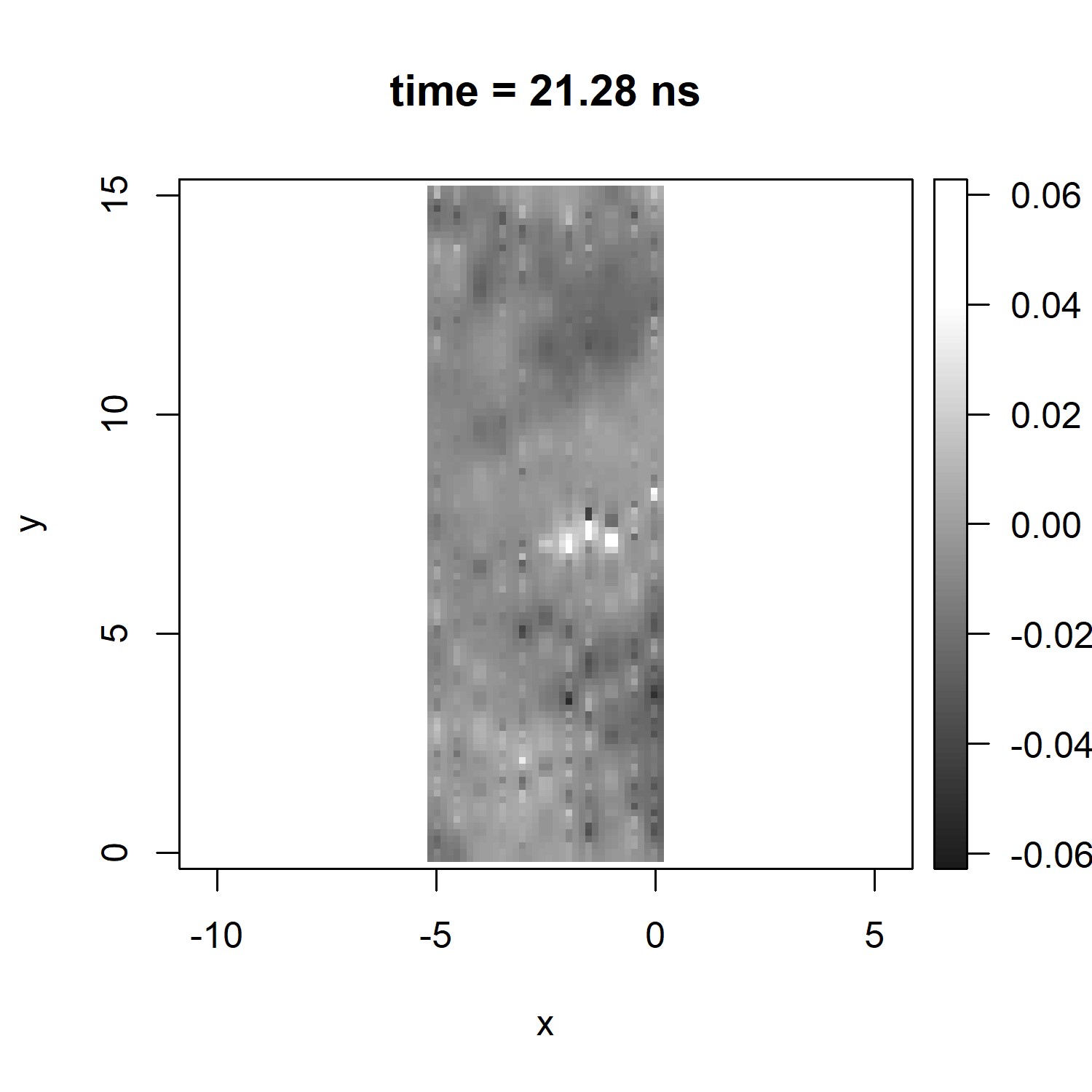
Finally, we can interpolate the lines and plot a slice:
SXY <- interpSlices(mySurvey, dx = 0.15, dy = 0.15, dz = 0.25, h = 10)

plot(SXY[,,120], col = palGPR("grey1"))
And a profile:
plot(mySurvey[[8]], relTime0 = TRUE, addFid = FALSE, col = palGPR("grey2"), ylim = c(14,67))
Readings#
Additional References#
Barba, L. and G. Pereira. 2003. Geophysical Study of Loma Guadalupe Archaeological Site in Michoacan, Mexico. Archaeologia Polona 41:118–122. https://doi.org/10.13140/RG.2.1.3177.8803
Barba, L., J. Blancas, A. Ortiz, and D. Carballo. 2009. Geophysical Prospection and Aerial Photography in La Laguna, Tlaxcala, Mexico. ArchéoSciences 33(suppl.):17–20. https://doi.org/10.4000/archeosciences.1194
Barba, L., J. Blancas, A. Ortiz, and J. Ligorred. 2009. GPR Detection of Karst and Archaeological Targets below the Historical Centre of Merida, Yucatán, Mexico. Studia Universitatis Babes-Bolyai, Geologia, 54(2):27–31. https://doi.org/10.5038/1937-8602.54.2.6
Campana, S., L. Marasco, A. Pecci, L. Barba, S. Piro, and D. Zamuner. 2009. Integration of Ground Remote Sensing Surveys and Archaeological Excavation to Characterize the Medieval Mound (Scarlino, Tuscany-Italy). ArchéoSciences 33(suppl.):133–135. https://doi.org/10.4000/archeosciences.1442
Conyers, L. B. 2006 Ground-Penetrating Radar. In Remote Sensing in Archaeology: An Explicitly North American Perspective, edited by J. K. Johnson. The University of Alabama Press, Alabama.
Daniels, Jr., J. T. 2014. Nondestructive Geophysical and Archaeometric Investigations at the Southern Belize Sites of Lubaantun and Nim Li Punit. University of California, San Diego.
Dixon, C. C. 2006. The use of Ground-Penetrating Radar to Detect Cultural Features: Ceren, El Salvador.
Gaffney, V. et al. 2018. Durrington Walls and the Stonehenge Hidden Landscape Project 2010–2016. Archaeological Prospection 25(3):255–269. https://doi.org/10.1002/arp.1707
Munro-Stasiuk, M. J. and T.K. Manahan. 2010. Investigating Ancient Maya Agricultural Adaptation through Ground-penetrating Radar (GPR) Analysis of Karst Terrain, Northern Yucatán, Mexico. Acta Carsologica 39(1):123–135. https://doi.org/10.3986/ac.v39i1.118
Pérez-Pérez, J., E.M.C. de Tapia, L. Barba-Pingarrón, J.E. Gama-Castro, and A. Peralta-Higuera. 2012. Remote Sensing Detection of Potential Sites in a Prehispanic Domestic Agricultural Terrace System in Cerro San Lucas, Teotihuacan, Mexico. Boletin de La Sociedad Geologica Mexicana 64(1):109–118. https://doi.org/10.18268/BSGM2012v64n1a9
Saey, T., M. Van Meirvenne, P. De Smedt, B. Stichelbaut, S. Delefortrie, E. Baldwin, and V. Gaffney. 2015. Combining EMI and GPR for Non-invasive Soil Sensing at the Stonehenge World Heritage Site: The Reconstruction of a WW1 Practice Trench. European Journal of Soil Science 66(1):166–178. https://doi.org/10.1111/ejss.12177
Safi, K. N., O.C. Mazariegos, C.P. Lipo, and H. Neff. 2012. Using Ground-Penetrating Radar to Examine Spatial Organization at the Late Classic Maya Site of El Baúl, Cotzumalhuapa, Guatemala. Geoarchaeology 27(5):410–425. https://doi.org/10.1002/gea.21414
Skaggs, S., T.G. Powis, C.R. Rucker, and G. Micheletti. 2016. An Iterative Approach to Ground Penetrating Radar at the Maya Site of Pacbitun, Belize. Remote Sensing 8(10):1–26. https://doi.org/10.3390/rs8100805
Valdés, J. A. and J. Kaplan. 2000. Ground-Penetrating Radar at the Maya Site of Kaminaljuyu, Guatemala. International Journal of Phytoremediation 21(1):329–342. https://doi.org/10.1179/jfa.2000.27.3.329
Verdonck, L., A. Launaro, F. Vermeulen, and M. Millett. 2020. Ground-Penetrating Radar Survey at Falerii Novi: A New Approach to the Study of Roman Cities. Antiquity 94(375):705–723. https://doi.org/10.15184/aqy.2020.82