Cell Statistics and Map Algebra

Map algebra is a fundamental concept in raster GIS, involving applying mathematical operations to one or more raster layers. In this technique, raster layers can be treated like variables in algebra to apply arithmetic, including addition, subtraction, division, averaging, etc.

Cell Statistics

The Cell Statistics tool calculates a per cell statistic across multiple rasters. When these rasters overlap, a statistic is applied to them to produce an output raster. When the rasters do not overlap, the rasters can be combined to increase the extent of data; for example, when combining several tiles of data (e.g., digital elevation models).

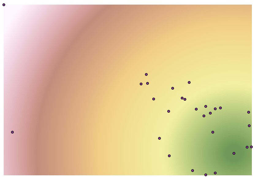
The following image shows a Euclidean distance accumulation based off a single point (representing an archaeological site):

Another raster layer below shows the same operation but over a different point or site:

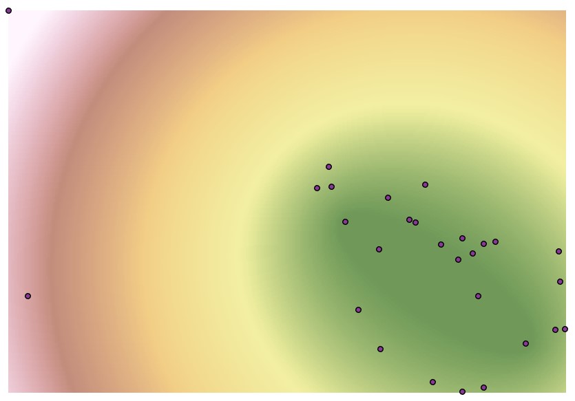
We can use the Cell Statistics tool to determine the minimum distance from either site. In the following raster layer, each cell represents the minimum distance to one of these two sites:

Alternatively, we could run Cell Statistics set to maximum, to determine the maximum distance to either of these two sites:

Or the mean:

Raster Calculator

The Cell Statistics tool has a limited number of mathematical operations. The Raster Calculator tool provides more flexibility in defining such operations.

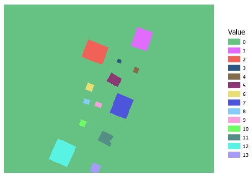
To illustrate, we can combine the following raster layers. The first layer represents architecture with values ranging from 1 to 13 over a background of 0:

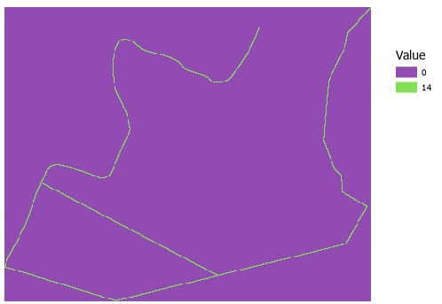
The second layer represents a road with a value of 14 over a background of 0:

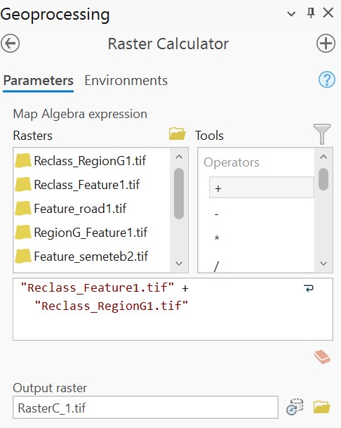
We could run the Cell Statistics tool with the statistic set to sum, or we could run Raster Calculator with the following formula, adding these two layers together:

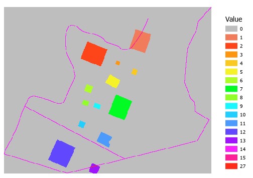
Doing so, we generate an output where 0 still represents the background, 1 to 13 still represent mounds, 14 still represents the road, but we now have additional values 15 and 27 that represent areas where the road overlaps architecture. In the case of 15, we have areas where the road overlaps the architecture with the value of 1, and in the case of 27, we have areas where the road overlaps the architecture with a value of 13:

We can also set Boolean operations, or true/false operations. If we run the following operation on the above output:

"input.tif"  <= 14

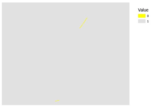
We get an image where values less than or equal to 14 have been set 1, and values above 14 have been set to 0, separating areas where the road crosses architecture:

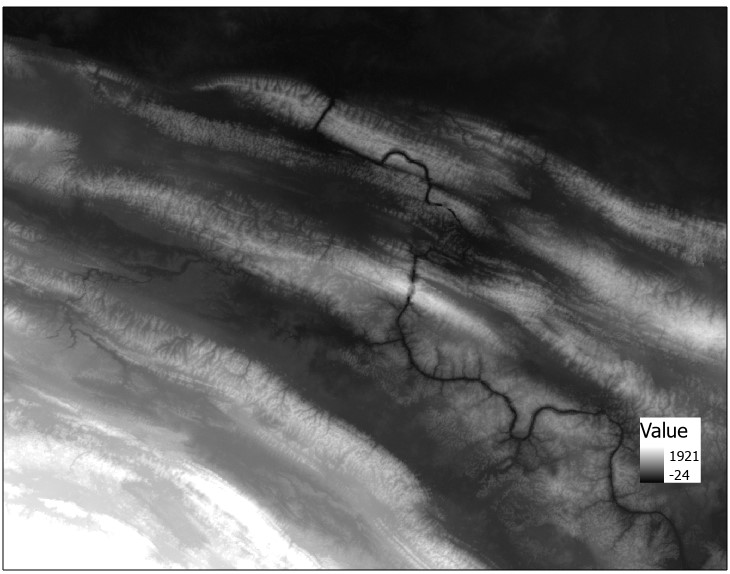
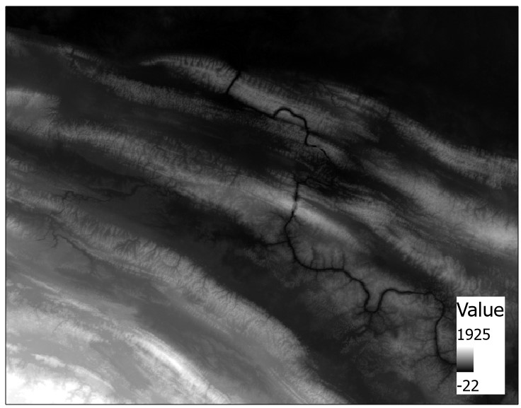
We can also set conditional statements. The following operation defines a conditional statement that where values in the DEM are less than 300, they should be set to 0, otherwise all other values should keep the same value in the raster.

Con("dem.tif" < 300, 0, "dem.tif")

When applied to the following DEM:

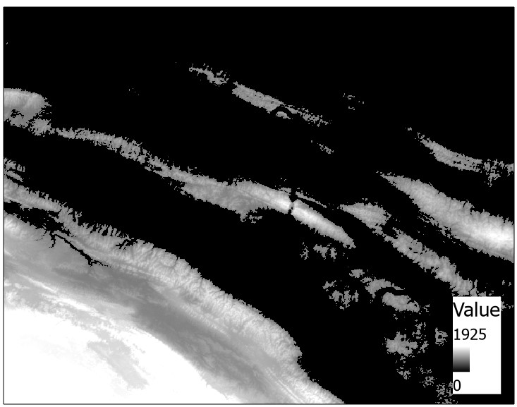
We get the following output:

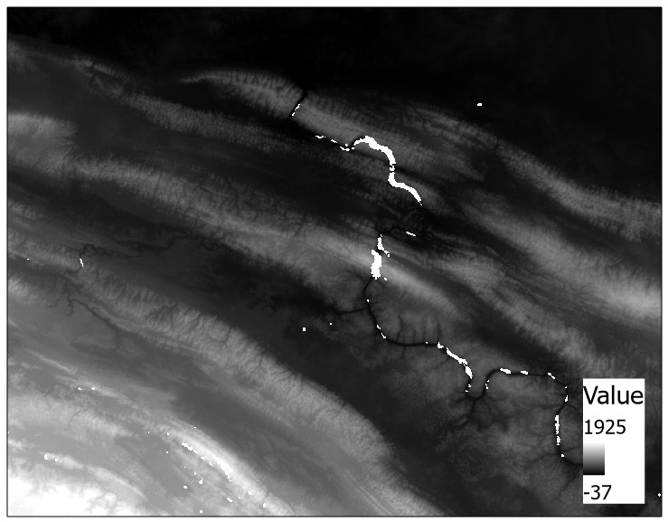
We can also use a conditional statement to replace NoData values with values from another raster. In the following example, we are filling the voids of a 1-arc second SRTM DEM with the values from a void-filled 3-arc second SRTM DEM. If we set the cell size under Environments to Minimum of Inputs, the output raster will be resampled to 1-arc second resolution.

Con(IsNull("1arc_dem.tif") , "3arc_dem.tif", "1arc_dem.tif")

Stated in plain English, this conditional statement can be read as “When the 1-arc second DEM has NoData, replace these values with those from the 3-arc second DEM, otherwise keep the 1-arc second DEM.”

The following raster layer represents the 1-arc second SRTM DEM with voids:

And the result of the raster calculator operation: