Introduction to Raster Tools#
Raster data in GIS refers to imagery displaying continuous data in pixels or cells. Rasters can be interpreted as tabular data where each pixel has a horizontal location, resolution, and a value (or digital number). The data is best visualized in this format when output as a text file, for example using the Raster to ASCII tool.
The following table represents a digital elevation model raster:
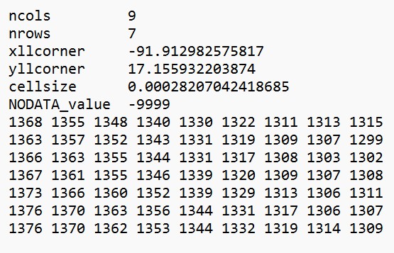
In this example, the table is defined by 9 columns and 7 rows. The location of the raster is defined by the coordinate of the lower left corner cell, and the resolution as cellsize (measured in degrees). The NODATA value is assigned the arbitrary value -9999. The additional values all represent the value of each pixel, each known as a digital number.
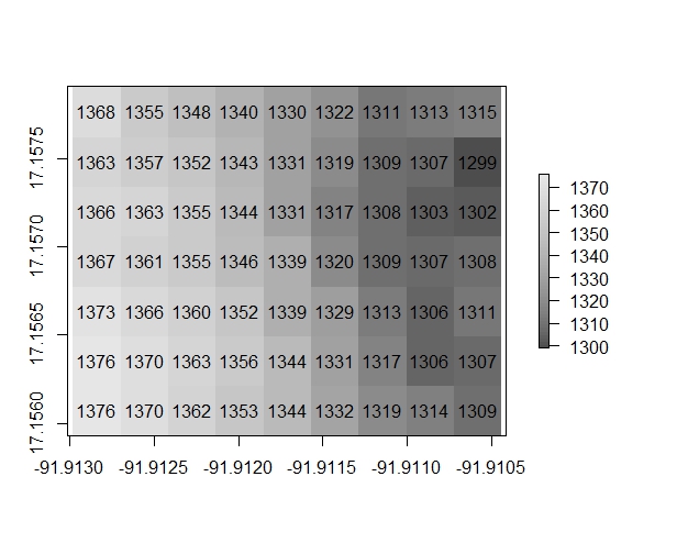
When viewed as an image, the digital elevation model has the following digital numbers displayed along a grayscale. Each digital number represents the elevation in meters at that location:
Here is another example, but this raster image represents a black and white photo where the digital numbers represent the relative brightness or darkness of the photo:

Source: https://gsp.humboldt.edu/olm/Courses/GSP_216/online/lesson5/raster-models.html
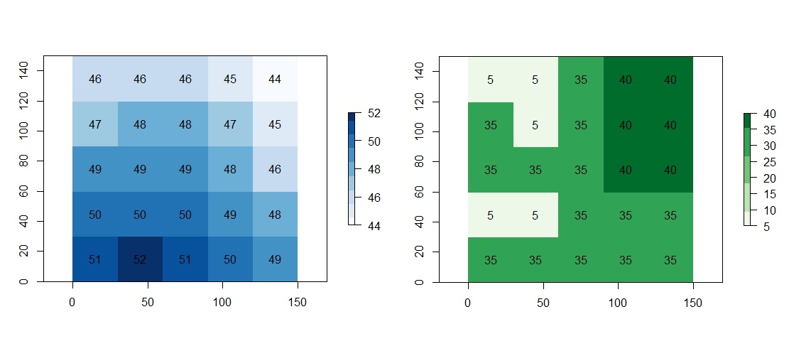
The following digital numbers represent inches of precipitation (left) and ground cover type (right). In the right example, the data are categorical rather than continuous.
No Data#
A critical concept in raster GIS is that at times no data is available in a particular cell. Note that No data is not the same as zero.
No data can occur when there is literally a gap in data at that specific location, or the data are outside the boundaries of the region of interest.
In the following example, the raster image is not rectangular:

However, the symbology here is misleading because, in reality, the raster image is rectangular. Under Symbology -> Mask, we can assign a background color (in this case black), which applies to No Data areas:
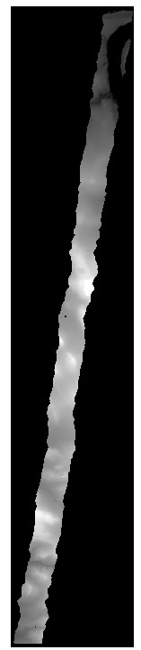
So, in fact, the raster is rectangular. Areas outside of the region of interest have been assigned No Data. In addition, we can also see that some areas inside the region of interest have the same No Data value. These are areas where no elevation data is available. If we use the Explore tool to identify the values in these locations, we will see they are assigned NoData.
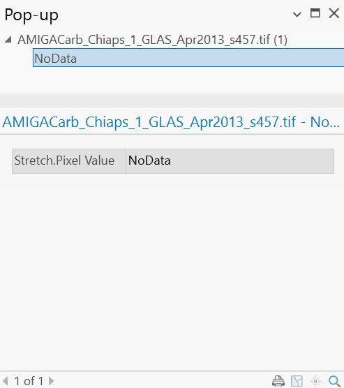
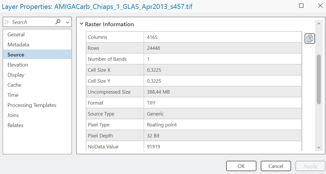
NoData, however, is not actually a numeric value but rather a character string. In reality, NoData values are assigned an actual numeric value. We can view this value by right-clicking the layer in Contents and opening Properties. Under Source -> Raster Information, we see in this case the NoData value is 91919:
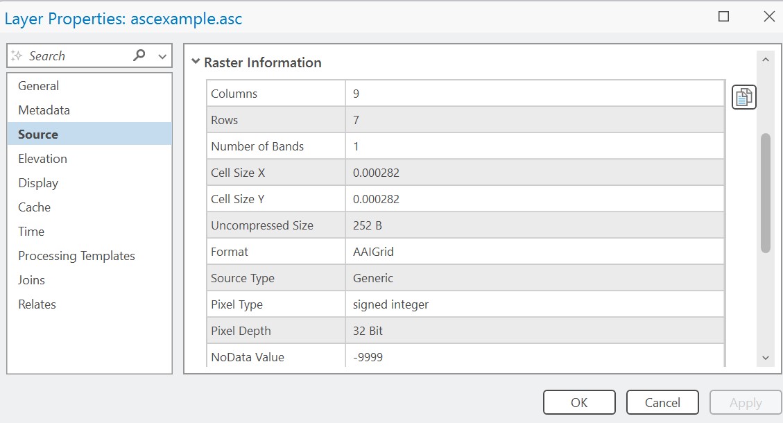
In our previous example above, however, we saw that NoData was assigned the value -9999:
NoData, therefore, must be defined with a numeric value. However, when defining NoData, we have to select a value that is outside of the range of our data. In the last two examples, we had not elevation data equal to 91,919 meters or -9,999 meters, so we could arbitrarily select those values to represent NoData. We cannot just choose any random value, however; we must ensure the value is within the bit depth of our raster.
Bit Depth#
We can also see additional information in the previous examples, namely pixel depth. In one example, pixel depth is 32 bit floating point and the other is 32 bit signed integer. These categories refer to the range of possible values in our rasters. Just as when we create a new field in a feature class attribute table or a standalone table, we have to define the type of data, including text, numeric, integer, or floating point (decimals). For raster, we can only define numeric values. The following are the most common bit depths seen in GIS. As a rule of thumb, we can calculate the range of possible values by raising 2 to the power of the bit.
1 Bit – 21 possible values, or 2 total values, only positive integers. This pixel depth represents binary data that stores only values of 0 and 1. If NoData were to be defined in this example, the value would have to be either 0 or 1, which would leave only a single possible value for the raster grid.
2 Bit – 22 possible values, or 4 total values, only positive integers. Data ranges from 0 to 3.
4 Bit – 24 possible values, or 16 total values, only positive integers. Data ranges from 0 to 15.
8 Bit unsigned – 28, or 256 total values, only positive integers. The range of 8 bit unsigned data is usually 0 to 255, with either 0 or 255 assigned to NoData. This pixel depth is most commonly used with grayscale photos and imagery (when using 3 bands, these data can be displayed with RGB values).
8 Bit signed – 28, or 256 total values, including negative and positive integers. The data range is -128 to 127. NoData could be assigned either -128 or 127.
16 Bit unsigned – 216, or 65,536 total values, only positive integers. The range is 0 to 65,535. NoData would likely be assigned either 0 or 65,535.
16 Bit signed – 216, or 65,536 total values, including negative and positive integers. The range is -32768 to 32767. In this example, NoData could be assigned the value -9999 because it is in range of the data.
32 Bit unsigned – 232, or 4,294,967,296 total values, only positive integers. The range is 0 to 4,294,967,295.
32 Bit signed – 232, or 4,294,967,296 total values, including negative and positive integers. The range is -2147483648 to 2147483647.
32 Bit float – 232, or 4,294,967,296 total values; the only pixel depth that can handle decimals. Data ranges from -3.402823466e+38 to 3.402823466e+38.
64 Bit unsigned – 264, or 18,446,744,073,709,551,616 total values, only positive integers. Data ranges from 0 to 18446744073709551616.
ArcGIS Pro will generally automatically select the appropriate pixel depth for the data being used, but it is useful to keep pixel depth in mind. Higher pixel depths take up more memory, and large rasters with a high pixel depth can be huge files, so use only the pixel depth necessary to contain your range of digital numbers. Note that 32 Bit float will likely be the most common pixel depth used, but 8 bit and 16 bit unsigned are also very common.